


备注
点击:ref:`这里 <sphx_glr_download_beginner_introyt_introyt1_tutorial.py>`下载完整示例代码
入门 || 张量 || 自动梯度 || 构建模型 || TensorBoard支持 || 训练模型 || 模型理解
PyTorch入门
Created On: Nov 30, 2021 | Last Updated: Jun 05, 2025 | Last Verified: Nov 05, 2024
可在以下视频中或在`YouTube上 <https://www.youtube.com/watch?v=IC0_FRiX-sw>`__观看。
PyTorch张量
从`03:50 <https://www.youtube.com/watch?v=IC0_FRiX-sw&t=230s>`__开始,观看以下视频。
首先,我们将导入 PyTorch。
import torch
让我们看看几个基本的张量操作。首先,是创建张量的几种方法:
z = torch.zeros(5, 3)
print(z)
print(z.dtype)
tensor([[0., 0., 0.],
        [0., 0., 0.],
        [0., 0., 0.],
        [0., 0., 0.],
        [0., 0., 0.]])
torch.float32
上面,我们创建了一个 5x3 的矩阵,填充为零,并查询其数据类型以发现这些零是 32 位浮点数,这是 PyTorch 的默认设置。
如果您想要整数怎么办?您始终可以覆盖默认设置:
i = torch.ones((5, 3), dtype=torch.int16)
print(i)
tensor([[1, 1, 1],
        [1, 1, 1],
        [1, 1, 1],
        [1, 1, 1],
        [1, 1, 1]], dtype=torch.int16)
您可以看到,当我们更改默认设置时,张量在打印时会显式地报告这一点。
在初始化学习权重时,通常会随机分配,通常带有特定的伪随机数种子以便于结果重现:
torch.manual_seed(1729)
r1 = torch.rand(2, 2)
print('A random tensor:')
print(r1)

r2 = torch.rand(2, 2)
print('\nA different random tensor:')
print(r2) # new values

torch.manual_seed(1729)
r3 = torch.rand(2, 2)
print('\nShould match r1:')
print(r3) # repeats values of r1 because of re-seed
A random tensor:
tensor([[0.3126, 0.3791],
        [0.3087, 0.0736]])

A different random tensor:
tensor([[0.4216, 0.0691],
        [0.2332, 0.4047]])

Should match r1:
tensor([[0.3126, 0.3791],
        [0.3087, 0.0736]])
PyTorch 张量直观地执行算术操作。形状相似的张量可以进行加法、乘法等操作。同标量的操作会分布到整个张量上:
ones = torch.ones(2, 3)
print(ones)

twos = torch.ones(2, 3) * 2 # every element is multiplied by 2
print(twos)

threes = ones + twos       # addition allowed because shapes are similar
print(threes)              # tensors are added element-wise
print(threes.shape)        # this has the same dimensions as input tensors

r1 = torch.rand(2, 3)
r2 = torch.rand(3, 2)
# uncomment this line to get a runtime error
# r3 = r1 + r2
tensor([[1., 1., 1.],
        [1., 1., 1.]])
tensor([[2., 2., 2.],
        [2., 2., 2.]])
tensor([[3., 3., 3.],
        [3., 3., 3.]])
torch.Size([2, 3])
以下是部分可用数学操作的简单示例:
r = (torch.rand(2, 2) - 0.5) * 2 # values between -1 and 1
print('A random matrix, r:')
print(r)

# Common mathematical operations are supported:
print('\nAbsolute value of r:')
print(torch.abs(r))

# ...as are trigonometric functions:
print('\nInverse sine of r:')
print(torch.asin(r))

# ...and linear algebra operations like determinant and singular value decomposition
print('\nDeterminant of r:')
print(torch.det(r))
print('\nSingular value decomposition of r:')
print(torch.svd(r))

# ...and statistical and aggregate operations:
print('\nAverage and standard deviation of r:')
print(torch.std_mean(r))
print('\nMaximum value of r:')
print(torch.max(r))
A random matrix, r:
tensor([[ 0.9956, -0.2232],
        [ 0.3858, -0.6593]])

Absolute value of r:
tensor([[0.9956, 0.2232],
        [0.3858, 0.6593]])

Inverse sine of r:
tensor([[ 1.4775, -0.2251],
        [ 0.3961, -0.7199]])

Determinant of r:
tensor(-0.5703)

Singular value decomposition of r:
torch.return_types.svd(
U=tensor([[-0.8353, -0.5497],
        [-0.5497,  0.8353]]),
S=tensor([1.1793, 0.4836]),
V=tensor([[-0.8851, -0.4654],
        [ 0.4654, -0.8851]]))

Average and standard deviation of r:
(tensor(0.7217), tensor(0.1247))

Maximum value of r:
tensor(0.9956)
关于 PyTorch 张量的强大功能还有很多需要了解,包括如何配置它们以在 GPU 上进行并行计算——我们将在另一部视频中深入探讨。
PyTorch 模型
从视频 10:00 开始跟随。
让我们讨论如何在 PyTorch 中表示模型。
import torch                     # for all things PyTorch
import torch.nn as nn            # for torch.nn.Module, the parent object for PyTorch models
import torch.nn.functional as F  # for the activation function
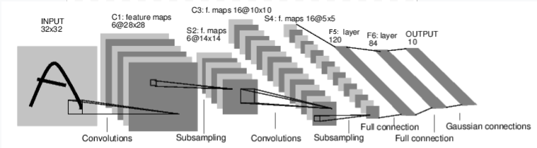
图:LeNet-5
上图是 LeNet-5 的示意图,这是最早的卷积神经网络之一,也是深度学习爆发的推动者之一。它用于读取小型手写数字图像(MNIST 数据集),并正确分类图像中表示的数字。
以下是其工作的简要说明:
C1 层是一个卷积层,意味着它扫描输入图像中在训练过程中学习到的特征。它输出一个激活图,表示图像中每个学习特征的位置。该“激活图”在 S2 层中被下采样。
C3 层是另一个卷积层,这次扫描 C1 的激活图以寻找*特征组合*。它还输出一个激活图,描述这些特征组合的空间位置,该图在 S4 层被下采样。
最后,末端的全连接层 F5、F6 和 OUTPUT 是*分类器*,它将最终的激活图分类为表示 10 个数字之一的十个分类。
我们如何用代码表示这个简单的神经网络?
class LeNet(nn.Module):

    def __init__(self):
        super(LeNet, self).__init__()
        # 1 input image channel (black & white), 6 output channels, 5x5 square convolution
        # kernel
        self.conv1 = nn.Conv2d(1, 6, 5)
        self.conv2 = nn.Conv2d(6, 16, 5)
        # an affine operation: y = Wx + b
        self.fc1 = nn.Linear(16 * 5 * 5, 120)  # 5*5 from image dimension
        self.fc2 = nn.Linear(120, 84)
        self.fc3 = nn.Linear(84, 10)

    def forward(self, x):
        # Max pooling over a (2, 2) window
        x = F.max_pool2d(F.relu(self.conv1(x)), (2, 2))
        # If the size is a square you can only specify a single number
        x = F.max_pool2d(F.relu(self.conv2(x)), 2)
        x = x.view(-1, self.num_flat_features(x))
        x = F.relu(self.fc1(x))
        x = F.relu(self.fc2(x))
        x = self.fc3(x)
        return x

    def num_flat_features(self, x):
        size = x.size()[1:]  # all dimensions except the batch dimension
        num_features = 1
        for s in size:
            num_features *= s
        return num_features
看一下这段代码,你应该能够发现它与上方示意图的一些结构相似之处。
这展示了一个典型 PyTorch 模型的结构:
它继承自
torch.nn.Module- 模块可以嵌套 - 实际上,连Conv2d和Linear层类也继承自torch.nn.Module。一个模型将拥有一个
__init__()函数,在这个函数中实例化其层,并加载任何它可能需要的数据资源(例如,一个 NLP 模型可能会加载词汇表)。一个模型还会有一个
forward()函数。这是实际计算发生的地方:输入经过网络层和各种函数处理以生成输出。除此之外,你可以像构建任何 Python 类一样构建你的模型类,添加任何支持模型计算所需的属性和方法。
让我们实例化这个对象并运行一个示例输入。
net = LeNet()
print(net)                         # what does the object tell us about itself?

input = torch.rand(1, 1, 32, 32)   # stand-in for a 32x32 black & white image
print('\nImage batch shape:')
print(input.shape)

output = net(input)                # we don't call forward() directly
print('\nRaw output:')
print(output)
print(output.shape)
LeNet(
  (conv1): Conv2d(1, 6, kernel_size=(5, 5), stride=(1, 1))
  (conv2): Conv2d(6, 16, kernel_size=(5, 5), stride=(1, 1))
  (fc1): Linear(in_features=400, out_features=120, bias=True)
  (fc2): Linear(in_features=120, out_features=84, bias=True)
  (fc3): Linear(in_features=84, out_features=10, bias=True)
)

Image batch shape:
torch.Size([1, 1, 32, 32])

Raw output:
tensor([[ 0.0898,  0.0318,  0.1485,  0.0301, -0.0085, -0.1135, -0.0296,  0.0164,
          0.0039,  0.0616]], grad_fn=<AddmmBackward0>)
torch.Size([1, 10])
上述操作中有几个关键点:
首先,我们实例化了 LeNet 类,并打印了 net 对象。torch.nn.Module 的子类会报告它已创建的层及其形状和参数。如果您想了解模型的处理过程概要,这可以提供一个方便的概述。
在下方,我们创建了一个表示 32x32 图像且有一个色彩通道的虚拟输入。通常情况下,你会加载一个图像块并将其转换为这种形状的张量。
你可能已经注意到我们的张量中有额外的维度 - 即批量维度。PyTorch 模型假设它们在处理数据的*批量*——例如,我们的图像块的一个包含 16 个样本的批量会有形状 (16, 1, 32, 32)。由于我们只使用一张图像,所以我们创建了一个批量大小为 1 的数据,形状为 (1, 1, 32, 32)。
我们通过调用模型来请求推理,就像调用一个函数一样:net(input)。这个调用的输出表示模型对输入表示某个特定数字的信心。(由于这个模型的实例尚未学到任何东西,所以我们不应该期望在输出中看到任何显著信号。)查看 output 的形状,我们可以看到它也有一个批量维度,其大小应该始终与输入批量维度匹配。如果我们传入一个包含 16 个实例的输入批量,output 的形状将为 (16, 10)。
数据集和数据加载器
从视频 14:00 开始跟随。
下面,我们将演示如何使用 TorchVision 中的一个可下载的开源数据集,如何转换图像以供模型使用,以及如何使用 DataLoader 将数据批量传递到模型中。
我们需要做的第一件事是将输入图像转换为 PyTorch 张量。
#%matplotlib inline

import torch
import torchvision
import torchvision.transforms as transforms

transform = transforms.Compose(
    [transforms.ToTensor(),
     transforms.Normalize((0.4914, 0.4822, 0.4465), (0.2470, 0.2435, 0.2616))])
这里,我们为输入指定了两个转换:
transforms.ToTensor()将通过 Pillow 加载的图像转换为 PyTorch 张量。transforms.Normalize()调整张量的值,使其平均值为零,标准差为 1.0。大多数激活函数在 x = 0 附近具有最强的梯度,因此将数据居中可以加速学习。传递给该转换的值是数据集中图像 rgb 值的平均值(第一个元组)和标准差(第二个元组)。您可以运行以下几行代码自己计算这些值:from torch.utils.data import ConcatDataset transform = transforms.Compose([transforms.ToTensor()]) trainset = torchvision.datasets.CIFAR10(root='./data', train=True, download=True, transform=transform) # stack all train images together into a tensor of shape # (50000, 3, 32, 32) x = torch.stack([sample[0] for sample in ConcatDataset([trainset])]) # get the mean of each channel mean = torch.mean(x, dim=(0,2,3)) # tensor([0.4914, 0.4822, 0.4465]) std = torch.std(x, dim=(0,2,3)) # tensor([0.2470, 0.2435, 0.2616])
还有许多其他可用的转换,包括裁剪、居中、旋转和反射。
接下来,我们将创建一个 CIFAR10 数据集实例。这是一个包含 32x32 彩色图像块的数据集,表示十种类别的对象:6 种动物(鸟、猫、鹿、狗、青蛙、马)和 4 种车辆(飞机、汽车、船、卡车):
trainset = torchvision.datasets.CIFAR10(root='./data', train=True,
                                        download=True, transform=transform)
  0%|          | 0.00/170M [00:00<?, ?B/s]
  0%|          | 32.8k/170M [00:00<42:09, 67.4kB/s]
  0%|          | 98.3k/170M [00:00<18:54, 150kB/s]
  0%|          | 197k/170M [00:00<11:34, 245kB/s]
  0%|          | 393k/170M [00:01<06:25, 441kB/s]
  0%|          | 819k/170M [00:01<03:14, 874kB/s]
  1%|          | 1.64M/170M [00:01<01:40, 1.68MB/s]
  2%|1         | 3.24M/170M [00:01<00:51, 3.22MB/s]
  4%|3         | 6.36M/170M [00:02<00:26, 6.19MB/s]
  6%|5         | 9.50M/170M [00:02<00:19, 8.24MB/s]
  7%|7         | 12.6M/170M [00:02<00:16, 9.65MB/s]
  9%|9         | 15.7M/170M [00:02<00:14, 10.6MB/s]
 11%|#1        | 18.9M/170M [00:03<00:13, 11.3MB/s]
 13%|#2        | 22.0M/170M [00:03<00:12, 11.8MB/s]
 15%|#4        | 25.1M/170M [00:03<00:12, 12.1MB/s]
 17%|#6        | 28.2M/170M [00:03<00:11, 12.3MB/s]
 18%|#8        | 31.4M/170M [00:04<00:11, 12.5MB/s]
 20%|##        | 34.5M/170M [00:04<00:10, 12.6MB/s]
 22%|##2       | 37.6M/170M [00:04<00:08, 15.3MB/s]
 23%|##3       | 39.4M/170M [00:04<00:09, 13.3MB/s]
 24%|##4       | 41.0M/170M [00:04<00:10, 11.9MB/s]
 26%|##5       | 43.6M/170M [00:04<00:08, 14.6MB/s]
 27%|##6       | 45.4M/170M [00:05<00:10, 12.4MB/s]
 28%|##7       | 47.0M/170M [00:05<00:10, 11.6MB/s]
 29%|##8       | 49.3M/170M [00:05<00:09, 13.4MB/s]
 30%|##9       | 50.8M/170M [00:05<00:10, 11.3MB/s]
 31%|###1      | 53.2M/170M [00:05<00:09, 12.2MB/s]
 33%|###2      | 55.5M/170M [00:05<00:08, 13.7MB/s]
 33%|###3      | 57.0M/170M [00:06<00:08, 12.8MB/s]
 34%|###4      | 58.6M/170M [00:06<00:08, 13.4MB/s]
 35%|###5      | 60.0M/170M [00:06<00:08, 12.6MB/s]
 36%|###6      | 61.7M/170M [00:06<00:08, 13.2MB/s]
 37%|###6      | 63.1M/170M [00:06<00:08, 12.4MB/s]
 38%|###7      | 64.7M/170M [00:06<00:08, 12.9MB/s]
 39%|###8      | 66.1M/170M [00:06<00:08, 12.3MB/s]
 40%|###9      | 67.9M/170M [00:06<00:07, 13.0MB/s]
 41%|####      | 69.2M/170M [00:07<00:08, 12.3MB/s]
 42%|####1     | 70.9M/170M [00:07<00:07, 13.0MB/s]
 42%|####2     | 72.3M/170M [00:07<00:08, 12.3MB/s]
 43%|####3     | 73.7M/170M [00:07<00:07, 12.8MB/s]
 44%|####4     | 75.0M/170M [00:07<00:07, 12.0MB/s]
 45%|####4     | 76.3M/170M [00:07<00:08, 11.7MB/s]
 46%|####5     | 78.2M/170M [00:07<00:07, 12.6MB/s]
 47%|####6     | 79.4M/170M [00:07<00:07, 12.0MB/s]
 48%|####7     | 81.3M/170M [00:08<00:06, 12.8MB/s]
 48%|####8     | 82.6M/170M [00:08<00:07, 12.2MB/s]
 49%|####9     | 84.4M/170M [00:08<00:06, 13.0MB/s]
 50%|#####     | 85.7M/170M [00:08<00:06, 12.2MB/s]
 51%|#####1    | 87.5M/170M [00:08<00:06, 13.1MB/s]
 52%|#####2    | 88.8M/170M [00:08<00:06, 12.1MB/s]
 53%|#####3    | 90.6M/170M [00:08<00:06, 13.2MB/s]
 54%|#####3    | 91.9M/170M [00:08<00:06, 11.6MB/s]
 55%|#####5    | 93.8M/170M [00:09<00:05, 13.4MB/s]
 56%|#####5    | 95.3M/170M [00:09<00:06, 11.7MB/s]
 57%|#####6    | 97.1M/170M [00:09<00:07, 10.4MB/s]
 59%|#####8    | 99.9M/170M [00:09<00:06, 10.8MB/s]
 60%|######    | 103M/170M [00:09<00:06, 11.1MB/s]
 62%|######1   | 106M/170M [00:10<00:05, 11.3MB/s]
 64%|######3   | 109M/170M [00:10<00:05, 11.4MB/s]
 65%|######5   | 111M/170M [00:10<00:05, 11.5MB/s]
 67%|######7   | 114M/170M [00:10<00:04, 11.8MB/s]
 69%|######8   | 118M/170M [00:11<00:04, 12.0MB/s]
 71%|#######   | 121M/170M [00:11<00:04, 12.2MB/s]
 73%|#######2  | 124M/170M [00:11<00:03, 12.3MB/s]
 74%|#######4  | 127M/170M [00:11<00:03, 12.4MB/s]
 76%|#######6  | 130M/170M [00:12<00:03, 12.5MB/s]
 78%|#######8  | 133M/170M [00:12<00:02, 12.5MB/s]
 80%|#######9  | 136M/170M [00:12<00:02, 12.5MB/s]
 82%|########1 | 139M/170M [00:12<00:02, 12.5MB/s]
 84%|########3 | 143M/170M [00:13<00:02, 12.5MB/s]
 85%|########5 | 146M/170M [00:13<00:01, 12.5MB/s]
 87%|########7 | 149M/170M [00:13<00:01, 12.4MB/s]
 89%|########9 | 152M/170M [00:13<00:01, 12.4MB/s]
 91%|######### | 155M/170M [00:14<00:01, 12.4MB/s]
 93%|#########2| 158M/170M [00:14<00:00, 12.5MB/s]
 94%|#########4| 161M/170M [00:14<00:00, 12.5MB/s]
 96%|#########6| 164M/170M [00:14<00:00, 12.5MB/s]
 98%|#########8| 167M/170M [00:15<00:00, 12.5MB/s]
100%|#########9| 170M/170M [00:15<00:00, 12.4MB/s]
100%|##########| 170M/170M [00:15<00:00, 11.1MB/s]
备注
运行上面的单元可能需要一点时间来下载数据集。
这是在 PyTorch 中创建数据集对象的一个示例。可下载的数据集(例如上方的 CIFAR-10)是 torch.utils.data.Dataset 的子类。PyTorch 中的 Dataset 类包括 TorchVision、Torchtext 和 TorchAudio 中的可下载数据集,以及诸如 torchvision.datasets.ImageFolder 之类的实用数据集类,它可以读取带标签的图像文件夹。您还可以创建自己的 Dataset 子类。
当我们实例化数据集时,需要告诉它几件事:
我们希望数据传输到的文件系统路径。
我们是否将此集用于训练;大多数数据集将被分为训练集和测试集。
如果我们尚未下载数据集,是否希望下载它。
我们希望对数据应用的转换。
一旦数据集准备好后,您可以将其提供给 DataLoader:
trainloader = torch.utils.data.DataLoader(trainset, batch_size=4,
                                          shuffle=True, num_workers=2)
Dataset 子类封装了对数据的访问,并专注于它所提供的数据类型。而 DataLoader 对数据一无所知,但会按照您指定的参数将 Dataset 提供的输入张量组织为批量。
在上面的示例中,我们要求 DataLoader 从 trainset 中给出批量大小为 4 的图像,随机化其顺序(shuffle=True),并让它启动两个工作线程从磁盘加载数据。
可视化您的 DataLoader 提供的批次是一个好习惯:
import matplotlib.pyplot as plt
import numpy as np

classes = ('plane', 'car', 'bird', 'cat',
           'deer', 'dog', 'frog', 'horse', 'ship', 'truck')

def imshow(img):
    img = img / 2 + 0.5     # unnormalize
    npimg = img.numpy()
    plt.imshow(np.transpose(npimg, (1, 2, 0)))


# get some random training images
dataiter = iter(trainloader)
images, labels = next(dataiter)

# show images
imshow(torchvision.utils.make_grid(images))
# print labels
print(' '.join('%5s' % classes[labels[j]] for j in range(4)))
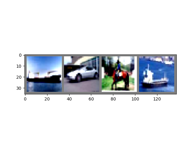
Clipping input data to the valid range for imshow with RGB data ([0..1] for floats or [0..255] for integers). Got range [-0.49473685..1.5632443].
 ship   car horse  ship
运行上面的单元格应显示四个图像的条形图,以及每个图像的正确标签。
训练您的 PyTorch 模型
从视频 17:10 开始跟随。
让我们将所有部分组合在一起,训练一个模型:
#%matplotlib inline

import torch
import torch.nn as nn
import torch.nn.functional as F
import torch.optim as optim

import torchvision
import torchvision.transforms as transforms

import matplotlib
import matplotlib.pyplot as plt
import numpy as np
首先,我们需要训练和测试数据集。如果您尚未下载,请运行下面的单元格以确保数据集已下载。(可能需要一分钟。)
transform = transforms.Compose(
    [transforms.ToTensor(),
     transforms.Normalize((0.5, 0.5, 0.5), (0.5, 0.5, 0.5))])

trainset = torchvision.datasets.CIFAR10(root='./data', train=True,
                                        download=True, transform=transform)
trainloader = torch.utils.data.DataLoader(trainset, batch_size=4,
                                          shuffle=True, num_workers=2)

testset = torchvision.datasets.CIFAR10(root='./data', train=False,
                                       download=True, transform=transform)
testloader = torch.utils.data.DataLoader(testset, batch_size=4,
                                         shuffle=False, num_workers=2)

classes = ('plane', 'car', 'bird', 'cat',
           'deer', 'dog', 'frog', 'horse', 'ship', 'truck')
我们将在 DataLoader 的输出上运行检查:
import matplotlib.pyplot as plt
import numpy as np

# functions to show an image


def imshow(img):
    img = img / 2 + 0.5     # unnormalize
    npimg = img.numpy()
    plt.imshow(np.transpose(npimg, (1, 2, 0)))


# get some random training images
dataiter = iter(trainloader)
images, labels = next(dataiter)

# show images
imshow(torchvision.utils.make_grid(images))
# print labels
print(' '.join('%5s' % classes[labels[j]] for j in range(4)))
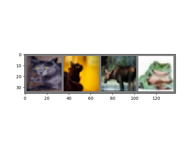
cat cat deer frog
这是我们将训练的模型。如果它看起来很熟悉,那是因为它是 LeNet 的一个变体 - 在本视频前面讨论过 - 适配了三色图像。
class Net(nn.Module):
    def __init__(self):
        super(Net, self).__init__()
        self.conv1 = nn.Conv2d(3, 6, 5)
        self.pool = nn.MaxPool2d(2, 2)
        self.conv2 = nn.Conv2d(6, 16, 5)
        self.fc1 = nn.Linear(16 * 5 * 5, 120)
        self.fc2 = nn.Linear(120, 84)
        self.fc3 = nn.Linear(84, 10)

    def forward(self, x):
        x = self.pool(F.relu(self.conv1(x)))
        x = self.pool(F.relu(self.conv2(x)))
        x = x.view(-1, 16 * 5 * 5)
        x = F.relu(self.fc1(x))
        x = F.relu(self.fc2(x))
        x = self.fc3(x)
        return x


net = Net()
我们需要的最后两个元素是损失函数和优化器:
criterion = nn.CrossEntropyLoss()
optimizer = optim.SGD(net.parameters(), lr=0.001, momentum=0.9)
如本视频前面讨论的那样,损失函数是衡量模型预测结果与理想输出之间距离的指标。交叉熵损失是像我们这样的分类模型的典型损失函数。
优化器 驱动学习。在这里,我们创建了一个实现*随机梯度下降*的优化器,这是一个更为直接的优化算法之一。除算法的参数(如学习率(lr)和动量)外,我们还传入了 net.parameters(),它是模型中所有学习权重的集合——这是优化器调整的部分。
最后,所有这些被组装成了训练循环。运行这段代码,因为它可能需要几分钟来执行:
for epoch in range(2):  # loop over the dataset multiple times

    running_loss = 0.0
    for i, data in enumerate(trainloader, 0):
        # get the inputs
        inputs, labels = data

        # zero the parameter gradients
        optimizer.zero_grad()

        # forward + backward + optimize
        outputs = net(inputs)
        loss = criterion(outputs, labels)
        loss.backward()
        optimizer.step()

        # print statistics
        running_loss += loss.item()
        if i % 2000 == 1999:    # print every 2000 mini-batches
            print('[%d, %5d] loss: %.3f' %
                  (epoch + 1, i + 1, running_loss / 2000))
            running_loss = 0.0

print('Finished Training')
[1,  2000] loss: 2.195
[1,  4000] loss: 1.878
[1,  6000] loss: 1.657
[1,  8000] loss: 1.577
[1, 10000] loss: 1.518
[1, 12000] loss: 1.460
[2,  2000] loss: 1.416
[2,  4000] loss: 1.366
[2,  6000] loss: 1.330
[2,  8000] loss: 1.328
[2, 10000] loss: 1.316
[2, 12000] loss: 1.256
Finished Training
这里我们只进行了**两个训练轮次**(第 1 行)——即训练数据集的两次遍历。每次遍历都有一个内循环,**迭代训练数据**(第 4 行),提供转换后的输入图像和其正确标签的批次。
**清零梯度**(第 9 行)是一个重要步骤。梯度在一个批次中累积;如果我们对每个批次未重置它们,它们将继续累积,这会提供不正确的梯度值,使学习变得不可能。
在第 12 行,我们**向模型请求预测**该批次。在接下来的行(第 13 行),我们计算损失——``outputs``(模型预测)与 ``labels``(正确输出)之间的差距。
在第 14 行,我们进行了 backward() 传播,计算将指导学习的梯度。
在第 15 行,优化器执行了一次学习步骤——它使用来自 backward() 调用的梯度,将学习权重朝它认为会减少损失的方向推进。
循环的其余部分对轮次编号、已完成的训练实例数量以及训练循环中的累计损失进行了一些轻度报告。
[1,  2000] loss: 2.235
[1,  4000] loss: 1.940
[1,  6000] loss: 1.713
[1,  8000] loss: 1.573
[1, 10000] loss: 1.507
[1, 12000] loss: 1.442
[2,  2000] loss: 1.378
[2,  4000] loss: 1.364
[2,  6000] loss: 1.349
[2,  8000] loss: 1.319
[2, 10000] loss: 1.284
[2, 12000] loss: 1.267
Finished Training
注意,损失值是单调下降的,这表明我们的模型在训练数据集上的性能持续提升。
作为最后一步,我们需要检查模型是否确实在进行*泛化*学习,而不是简单地“记住”数据集。这被称为**过拟合**,通常意味着数据集太小(没有足够的示例进行泛化学习),或者模型拥有比正确建模数据集所需更多的学习参数。
这就是为什么数据集会被划分为训练和测试子集——为了测试模型的泛化能力,我们让它对未训练过的数据进行预测:
correct = 0
total = 0
with torch.no_grad():
    for data in testloader:
        images, labels = data
        outputs = net(images)
        _, predicted = torch.max(outputs.data, 1)
        total += labels.size(0)
        correct += (predicted == labels).sum().item()

print('Accuracy of the network on the 10000 test images: %d %%' % (
    100 * correct / total))
Accuracy of the network on the 10000 test images: 54 %
如果你跟随操作,你应该看到模型在这一点上的准确率大约是50%。这虽然不是最先进的水平,但远远好于随机输出的10%准确率。这表明模型确实发生了一些泛化学习。
