


备注
点击 :ref:`此处 <sphx_glr_download_beginner_transfer_learning_tutorial.py>`下载完整示例代码
计算机视觉迁移学习教程
Created On: Mar 24, 2017 | Last Updated: Jan 27, 2025 | Last Verified: Nov 05, 2024
在本教程中,您将学习如何使用迁移学习训练一个用于图像分类的卷积神经网络。您可以在`cs231n notes <https://cs231n.github.io/transfer-learning/>`__中阅读更多关于迁移学习的信息。
引述这些笔记,
实际上,很少有人从头开始(随机初始化)训练整个卷积网络,因为很少有大小足够的数据集。相反,通常会在一个非常大的数据集(例如包含1000个类别、120万张图像的ImageNet)上预训练一个卷积网络,然后将其用作初始化或固定的特征提取器来处理感兴趣的任务。
这两种主要的迁移学习场景如下:
微调卷积网络:与随机初始化不同,我们使用一个预训练的网络(如在imagenet 1000数据集上训练的网络)进行初始化,其余的训练过程与通常一致。
卷积网络作为固定特征提取器:在此处,我们将冻结除最后一个全连接层以外的所有网络权重。最后这个全连接层将被替换为一个具有随机权重的新层,仅训练这个层。
# License: BSD
# Author: Sasank Chilamkurthy

import torch
import torch.nn as nn
import torch.optim as optim
from torch.optim import lr_scheduler
import torch.backends.cudnn as cudnn
import numpy as np
import torchvision
from torchvision import datasets, models, transforms
import matplotlib.pyplot as plt
import time
import os
from PIL import Image
from tempfile import TemporaryDirectory

cudnn.benchmark = True
plt.ion()   # interactive mode
<contextlib.ExitStack object at 0x7f057d00b820>
加载数据
我们将使用torchvision和torch.utils.data包来加载数据。
今天我们要解决的问题是训练一个模型来分类**蚂蚁**和**蜜蜂**。我们每个类别大约有120张训练图片,每个类别有75张验证图片。通常情况下,从头训练这是一个很小的数据集,不足以进行泛化。由于我们使用迁移学习,我们应该能够做到合理泛化。
这个数据集是Imagenet的一个小子集。
备注
从`这里 <https://download.pytorch.org/tutorial/hymenoptera_data.zip>`_下载数据并将其解压到当前目录。
# Data augmentation and normalization for training
# Just normalization for validation
data_transforms = {
    'train': transforms.Compose([
        transforms.RandomResizedCrop(224),
        transforms.RandomHorizontalFlip(),
        transforms.ToTensor(),
        transforms.Normalize([0.485, 0.456, 0.406], [0.229, 0.224, 0.225])
    ]),
    'val': transforms.Compose([
        transforms.Resize(256),
        transforms.CenterCrop(224),
        transforms.ToTensor(),
        transforms.Normalize([0.485, 0.456, 0.406], [0.229, 0.224, 0.225])
    ]),
}

data_dir = 'data/hymenoptera_data'
image_datasets = {x: datasets.ImageFolder(os.path.join(data_dir, x),
                                          data_transforms[x])
                  for x in ['train', 'val']}
dataloaders = {x: torch.utils.data.DataLoader(image_datasets[x], batch_size=4,
                                             shuffle=True, num_workers=4)
              for x in ['train', 'val']}
dataset_sizes = {x: len(image_datasets[x]) for x in ['train', 'val']}
class_names = image_datasets['train'].classes

# We want to be able to train our model on an `accelerator <https://pytorch.org/docs/stable/torch.html#accelerators>`__
# such as CUDA, MPS, MTIA, or XPU. If the current accelerator is available, we will use it. Otherwise, we use the CPU.

device = torch.accelerator.current_accelerator().type if torch.accelerator.is_available() else "cpu"
print(f"Using {device} device")
Using cuda device
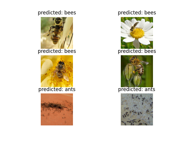
可视化一些图片
让我们可视化一些训练图片,以了解数据增强。
def imshow(inp, title=None):
    """Display image for Tensor."""
    inp = inp.numpy().transpose((1, 2, 0))
    mean = np.array([0.485, 0.456, 0.406])
    std = np.array([0.229, 0.224, 0.225])
    inp = std * inp + mean
    inp = np.clip(inp, 0, 1)
    plt.imshow(inp)
    if title is not None:
        plt.title(title)
    plt.pause(0.001)  # pause a bit so that plots are updated


# Get a batch of training data
inputs, classes = next(iter(dataloaders['train']))

# Make a grid from batch
out = torchvision.utils.make_grid(inputs)

imshow(out, title=[class_names[x] for x in classes])
![['bees', 'ants', 'bees', 'bees']](../_images/sphx_glr_transfer_learning_tutorial_001.png)
训练模型
现在,让我们编写一个通用函数来训练模型。这里,我们将说明:
调整学习率
保存最佳模型
在下面的内容中,参数``scheduler``是``torch.optim.lr_scheduler``中的一个LR调度对象。
def train_model(model, criterion, optimizer, scheduler, num_epochs=25):
    since = time.time()

    # Create a temporary directory to save training checkpoints
    with TemporaryDirectory() as tempdir:
        best_model_params_path = os.path.join(tempdir, 'best_model_params.pt')

        torch.save(model.state_dict(), best_model_params_path)
        best_acc = 0.0

        for epoch in range(num_epochs):
            print(f'Epoch {epoch}/{num_epochs - 1}')
            print('-' * 10)

            # Each epoch has a training and validation phase
            for phase in ['train', 'val']:
                if phase == 'train':
                    model.train()  # Set model to training mode
                else:
                    model.eval()   # Set model to evaluate mode

                running_loss = 0.0
                running_corrects = 0

                # Iterate over data.
                for inputs, labels in dataloaders[phase]:
                    inputs = inputs.to(device)
                    labels = labels.to(device)

                    # zero the parameter gradients
                    optimizer.zero_grad()

                    # forward
                    # track history if only in train
                    with torch.set_grad_enabled(phase == 'train'):
                        outputs = model(inputs)
                        _, preds = torch.max(outputs, 1)
                        loss = criterion(outputs, labels)

                        # backward + optimize only if in training phase
                        if phase == 'train':
                            loss.backward()
                            optimizer.step()

                    # statistics
                    running_loss += loss.item() * inputs.size(0)
                    running_corrects += torch.sum(preds == labels.data)
                if phase == 'train':
                    scheduler.step()

                epoch_loss = running_loss / dataset_sizes[phase]
                epoch_acc = running_corrects.double() / dataset_sizes[phase]

                print(f'{phase} Loss: {epoch_loss:.4f} Acc: {epoch_acc:.4f}')

                # deep copy the model
                if phase == 'val' and epoch_acc > best_acc:
                    best_acc = epoch_acc
                    torch.save(model.state_dict(), best_model_params_path)

            print()

        time_elapsed = time.time() - since
        print(f'Training complete in {time_elapsed // 60:.0f}m {time_elapsed % 60:.0f}s')
        print(f'Best val Acc: {best_acc:4f}')

        # load best model weights
        model.load_state_dict(torch.load(best_model_params_path, weights_only=True))
    return model
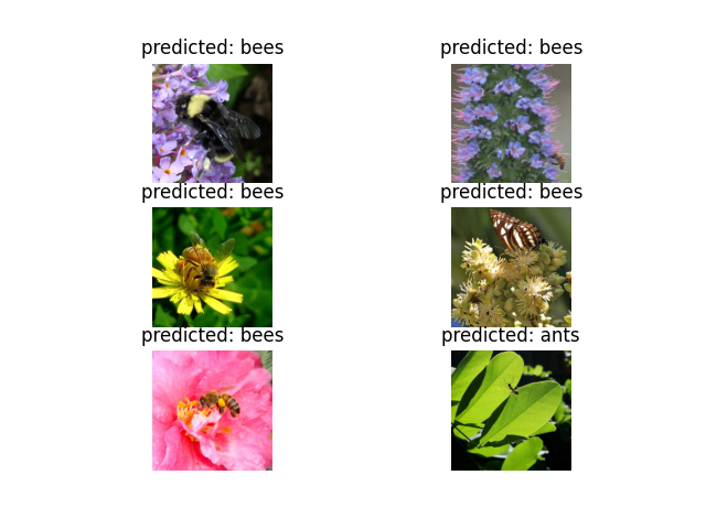
可视化模型预测
用于显示一些图片预测结果的通用功能
def visualize_model(model, num_images=6):
    was_training = model.training
    model.eval()
    images_so_far = 0
    fig = plt.figure()

    with torch.no_grad():
        for i, (inputs, labels) in enumerate(dataloaders['val']):
            inputs = inputs.to(device)
            labels = labels.to(device)

            outputs = model(inputs)
            _, preds = torch.max(outputs, 1)

            for j in range(inputs.size()[0]):
                images_so_far += 1
                ax = plt.subplot(num_images//2, 2, images_so_far)
                ax.axis('off')
                ax.set_title(f'predicted: {class_names[preds[j]]}')
                imshow(inputs.cpu().data[j])

                if images_so_far == num_images:
                    model.train(mode=was_training)
                    return
        model.train(mode=was_training)
微调卷积网络
加载一个预训练模型并重置最终全连接层。
model_ft = models.resnet18(weights='IMAGENET1K_V1')
num_ftrs = model_ft.fc.in_features
# Here the size of each output sample is set to 2.
# Alternatively, it can be generalized to ``nn.Linear(num_ftrs, len(class_names))``.
model_ft.fc = nn.Linear(num_ftrs, 2)

model_ft = model_ft.to(device)

criterion = nn.CrossEntropyLoss()

# Observe that all parameters are being optimized
optimizer_ft = optim.SGD(model_ft.parameters(), lr=0.001, momentum=0.9)

# Decay LR by a factor of 0.1 every 7 epochs
exp_lr_scheduler = lr_scheduler.StepLR(optimizer_ft, step_size=7, gamma=0.1)
Downloading: "https://download.pytorch.org/models/resnet18-f37072fd.pth" to /home/user/.cache/torch/hub/checkpoints/resnet18-f37072fd.pth

  0%|          | 0.00/44.7M [00:00<?, ?B/s]
  0%|          | 128k/44.7M [00:00<01:42, 458kB/s]
  1%|          | 256k/44.7M [00:00<01:04, 722kB/s]
  1%|1         | 512k/44.7M [00:00<00:37, 1.23MB/s]
  2%|2         | 1.00M/44.7M [00:00<00:20, 2.27MB/s]
  4%|4         | 1.88M/44.7M [00:00<00:10, 4.13MB/s]
  8%|7         | 3.38M/44.7M [00:00<00:05, 7.34MB/s]
 13%|#3        | 6.00M/44.7M [00:00<00:03, 13.0MB/s]
 19%|#8        | 8.38M/44.7M [00:01<00:02, 16.3MB/s]
 24%|##4       | 10.8M/44.7M [00:01<00:01, 18.6MB/s]
 30%|##9       | 13.2M/44.7M [00:01<00:01, 20.6MB/s]
 35%|###5      | 15.8M/44.7M [00:01<00:01, 22.0MB/s]
 41%|####1     | 18.4M/44.7M [00:01<00:01, 23.1MB/s]
 46%|####6     | 20.8M/44.7M [00:01<00:01, 23.4MB/s]
 52%|#####2    | 23.2M/44.7M [00:01<00:00, 23.9MB/s]
 58%|#####7    | 25.8M/44.7M [00:01<00:00, 24.3MB/s]
 63%|######3   | 28.2M/44.7M [00:01<00:00, 24.6MB/s]
 69%|######8   | 30.8M/44.7M [00:01<00:00, 24.7MB/s]
 74%|#######4  | 33.2M/44.7M [00:02<00:00, 25.0MB/s]
 80%|########  | 35.8M/44.7M [00:02<00:00, 25.1MB/s]
 86%|########5 | 38.2M/44.7M [00:02<00:00, 25.1MB/s]
 91%|#########1| 40.8M/44.7M [00:02<00:00, 24.7MB/s]
 97%|#########6| 43.2M/44.7M [00:02<00:00, 25.2MB/s]
100%|##########| 44.7M/44.7M [00:02<00:00, 18.2MB/s]
训练和评估
在CPU上大约需要15-25分钟。在GPU上,运行速度不到一分钟。
model_ft = train_model(model_ft, criterion, optimizer_ft, exp_lr_scheduler,
                       num_epochs=25)
Epoch 0/24
----------
train Loss: 0.5939 Acc: 0.7213
val Loss: 0.3330 Acc: 0.8562

Epoch 1/24
----------
train Loss: 0.7067 Acc: 0.7254
val Loss: 0.3340 Acc: 0.9085

Epoch 2/24
----------
train Loss: 0.4502 Acc: 0.8443
val Loss: 0.4508 Acc: 0.8366

Epoch 3/24
----------
train Loss: 0.6951 Acc: 0.7418
val Loss: 0.3874 Acc: 0.9085

Epoch 4/24
----------
train Loss: 0.6182 Acc: 0.7869
val Loss: 0.3596 Acc: 0.8954

Epoch 5/24
----------
train Loss: 0.5027 Acc: 0.7828
val Loss: 0.3200 Acc: 0.8693

Epoch 6/24
----------
train Loss: 0.4125 Acc: 0.8566
val Loss: 0.3906 Acc: 0.8497

Epoch 7/24
----------
train Loss: 0.5737 Acc: 0.7746
val Loss: 0.2773 Acc: 0.9085

Epoch 8/24
----------
train Loss: 0.3708 Acc: 0.8238
val Loss: 0.2560 Acc: 0.8954

Epoch 9/24
----------
train Loss: 0.4026 Acc: 0.8156
val Loss: 0.2561 Acc: 0.9150

Epoch 10/24
----------
train Loss: 0.2558 Acc: 0.9057
val Loss: 0.2645 Acc: 0.9150

Epoch 11/24
----------
train Loss: 0.3397 Acc: 0.8402
val Loss: 0.2506 Acc: 0.9020

Epoch 12/24
----------
train Loss: 0.4139 Acc: 0.8238
val Loss: 0.2763 Acc: 0.8889

Epoch 13/24
----------
train Loss: 0.2291 Acc: 0.9180
val Loss: 0.2511 Acc: 0.9281

Epoch 14/24
----------
train Loss: 0.3079 Acc: 0.8648
val Loss: 0.2608 Acc: 0.9150

Epoch 15/24
----------
train Loss: 0.3187 Acc: 0.8484
val Loss: 0.2566 Acc: 0.9216

Epoch 16/24
----------
train Loss: 0.3709 Acc: 0.8566
val Loss: 0.2324 Acc: 0.9216

Epoch 17/24
----------
train Loss: 0.2958 Acc: 0.8730
val Loss: 0.2485 Acc: 0.9216

Epoch 18/24
----------
train Loss: 0.3991 Acc: 0.8115
val Loss: 0.2497 Acc: 0.9085

Epoch 19/24
----------
train Loss: 0.2777 Acc: 0.8730
val Loss: 0.2496 Acc: 0.9281

Epoch 20/24
----------
train Loss: 0.2504 Acc: 0.9057
val Loss: 0.2480 Acc: 0.9085

Epoch 21/24
----------
train Loss: 0.2879 Acc: 0.8770
val Loss: 0.2475 Acc: 0.9281

Epoch 22/24
----------
train Loss: 0.2626 Acc: 0.9098
val Loss: 0.2489 Acc: 0.9281

Epoch 23/24
----------
train Loss: 0.3855 Acc: 0.8320
val Loss: 0.2574 Acc: 0.9281

Epoch 24/24
----------
train Loss: 0.3218 Acc: 0.8443
val Loss: 0.2607 Acc: 0.9150

Training complete in 0m 37s
Best val Acc: 0.928105
visualize_model(model_ft)
卷积网络作为固定特征提取器
在这篇教程中,我们需要冻结除最后一层之外的所有网络层。我们需要设置``requires_grad = False``以冻结参数,这样在``backward()``中就不会计算梯度。
您可以在`这里 <https://pytorch.org/docs/notes/autograd.html#excluding-subgraphs-from-backward>`__的文档中了解更多这方面内容。
model_conv = torchvision.models.resnet18(weights='IMAGENET1K_V1')
for param in model_conv.parameters():
    param.requires_grad = False

# Parameters of newly constructed modules have requires_grad=True by default
num_ftrs = model_conv.fc.in_features
model_conv.fc = nn.Linear(num_ftrs, 2)

model_conv = model_conv.to(device)

criterion = nn.CrossEntropyLoss()

# Observe that only parameters of final layer are being optimized as
# opposed to before.
optimizer_conv = optim.SGD(model_conv.fc.parameters(), lr=0.001, momentum=0.9)

# Decay LR by a factor of 0.1 every 7 epochs
exp_lr_scheduler = lr_scheduler.StepLR(optimizer_conv, step_size=7, gamma=0.1)
训练和评估
在CPU上该方法与之前比可以节约一半时间。这是预期之中的,因为大部分网络不需要计算梯度。但前向传播仍需要计算。
model_conv = train_model(model_conv, criterion, optimizer_conv,
                         exp_lr_scheduler, num_epochs=25)
Epoch 0/24
----------
train Loss: 0.5459 Acc: 0.7049
val Loss: 0.2753 Acc: 0.8693

Epoch 1/24
----------
train Loss: 0.3994 Acc: 0.8115
val Loss: 0.1870 Acc: 0.9412

Epoch 2/24
----------
train Loss: 0.5364 Acc: 0.7500
val Loss: 0.1839 Acc: 0.9477

Epoch 3/24
----------
train Loss: 0.5437 Acc: 0.7787
val Loss: 0.2447 Acc: 0.9346

Epoch 4/24
----------
train Loss: 0.4482 Acc: 0.8320
val Loss: 0.4642 Acc: 0.8301

Epoch 5/24
----------
train Loss: 0.7146 Acc: 0.7418
val Loss: 0.3052 Acc: 0.8954

Epoch 6/24
----------
train Loss: 0.4757 Acc: 0.7828
val Loss: 0.3576 Acc: 0.8758

Epoch 7/24
----------
train Loss: 0.4499 Acc: 0.7869
val Loss: 0.2039 Acc: 0.9477

Epoch 8/24
----------
train Loss: 0.3540 Acc: 0.8320
val Loss: 0.2187 Acc: 0.9412

Epoch 9/24
----------
train Loss: 0.4232 Acc: 0.8361
val Loss: 0.2496 Acc: 0.9281

Epoch 10/24
----------
train Loss: 0.3847 Acc: 0.8402
val Loss: 0.2050 Acc: 0.9542

Epoch 11/24
----------
train Loss: 0.3180 Acc: 0.8361
val Loss: 0.1998 Acc: 0.9542

Epoch 12/24
----------
train Loss: 0.3467 Acc: 0.8525
val Loss: 0.2066 Acc: 0.9542

Epoch 13/24
----------
train Loss: 0.3432 Acc: 0.8361
val Loss: 0.2050 Acc: 0.9412

Epoch 14/24
----------
train Loss: 0.3425 Acc: 0.8648
val Loss: 0.2116 Acc: 0.9477

Epoch 15/24
----------
train Loss: 0.3370 Acc: 0.8730
val Loss: 0.2015 Acc: 0.9477

Epoch 16/24
----------
train Loss: 0.3459 Acc: 0.8484
val Loss: 0.2037 Acc: 0.9412

Epoch 17/24
----------
train Loss: 0.3403 Acc: 0.8484
val Loss: 0.2261 Acc: 0.9412

Epoch 18/24
----------
train Loss: 0.3695 Acc: 0.8402
val Loss: 0.2046 Acc: 0.9477

Epoch 19/24
----------
train Loss: 0.2609 Acc: 0.8893
val Loss: 0.2018 Acc: 0.9477

Epoch 20/24
----------
train Loss: 0.3822 Acc: 0.8566
val Loss: 0.2069 Acc: 0.9542

Epoch 21/24
----------
train Loss: 0.3986 Acc: 0.8443
val Loss: 0.2108 Acc: 0.9412

Epoch 22/24
----------
train Loss: 0.3624 Acc: 0.8361
val Loss: 0.1925 Acc: 0.9477

Epoch 23/24
----------
train Loss: 0.3893 Acc: 0.8443
val Loss: 0.2048 Acc: 0.9412

Epoch 24/24
----------
train Loss: 0.3172 Acc: 0.8361
val Loss: 0.2318 Acc: 0.9346

Training complete in 0m 27s
Best val Acc: 0.954248
visualize_model(model_conv)

plt.ioff()
plt.show()
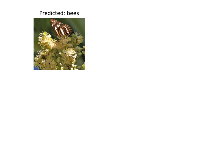
自定义图片推断
使用训练好的模型对自定义图片进行预测,并可视化带有预测类别标签的图片。
def visualize_model_predictions(model,img_path):
    was_training = model.training
    model.eval()

    img = Image.open(img_path)
    img = data_transforms['val'](img)
    img = img.unsqueeze(0)
    img = img.to(device)

    with torch.no_grad():
        outputs = model(img)
        _, preds = torch.max(outputs, 1)

        ax = plt.subplot(2,2,1)
        ax.axis('off')
        ax.set_title(f'Predicted: {class_names[preds[0]]}')
        imshow(img.cpu().data[0])

        model.train(mode=was_training)
visualize_model_predictions(
    model_conv,
    img_path='data/hymenoptera_data/val/bees/72100438_73de9f17af.jpg'
)

plt.ioff()
plt.show()
进一步学习
如果您想了解有关迁移学习应用的更多信息,请查看我们的`量化迁移学习用于计算机视觉教程 <https://pytorch.org/tutorials/intermediate/quantized_transfer_learning_tutorial.html>`_。
