使用Ax进行多目标NAS

Created On: Aug 19, 2022 | Last Updated: Jul 31, 2024 | Last Verified: Nov 05, 2024

作者: David Eriksson, Max Balandat, 和Meta的自适应实验团队。

在本教程中，我们展示了如何使用`Ax <https://ax.dev/>`__进行多目标神经架构搜索（NAS），以优化一个简单的神经网络模型在流行的MNIST数据集上的性能。虽然这种方法通常适用于更复杂的模型和更大的数据集，但我们选择了一个可以在笔记本电脑上少于20分钟内完整运行的教程。

在许多NAS应用中，多个感兴趣目标之间存在自然权衡。例如，在设备上部署模型时，我们可能希望最大化模型性能（如准确性），同时最小化诸如功耗、推理延迟或模型大小等竞争性指标，以满足部署约束条件。通常，我们可能通过接受稍微较低的模型性能，来显著减少计算需求或预测的延迟。高效探索这类权衡的系统方法是可扩展和可持续AI的重要推动因素，并在Meta有着许多成功应用 - 例如，请参阅我们关于自然语言理解模型的`案例研究 <https://research.facebook.com/blog/2021/07/optimizing-model-accuracy-and-latency-using-bayesian-multi-objective-neural-architecture-search/>`__。

在这个示例中，我们将调整两个隐藏层的宽度、学习率、丢弃概率、批量大小以及训练周期的数量。目标是在性能（验证集上的准确性）和模型大小（模型参数的数量）之间进行权衡。

本教程使用了以下PyTorch库：

• `PyTorch Lightning <https://github.com/PyTorchLightning/pytorch-lightning>`__（指定模型和训练循环）

• `TorchX <https://github.com/pytorch/torchx>`__（用于远程/异步运行训练作业）

• `BoTorch <https://github.com/pytorch/botorch>`__（支持Ax算法的贝叶斯优化库）

定义TorchX应用程序

我们的目标是优化在`mnist_train_nas.py <https://github.com/pytorch/tutorials/tree/main/intermediate_source/mnist_train_nas.py>`__中定义的PyTorch Lightning训练作业。为此，在使用TorchX时，我们编写了一个辅助函数，该函数接收训练作业的架构和值超参数，并创建一个具有适当设置的`TorchX AppDef <https://pytorch.org/torchx/latest/basics.html>`__。

from pathlib import Path

import torchx

from torchx import specs
from torchx.components import utils


def trainer(
    log_path: str,
    hidden_size_1: int,
    hidden_size_2: int,
    learning_rate: float,
    epochs: int,
    dropout: float,
    batch_size: int,
    trial_idx: int = -1,
) -> specs.AppDef:

    # define the log path so we can pass it to the TorchX ``AppDef``
    if trial_idx >= 0:
        log_path = Path(log_path).joinpath(str(trial_idx)).absolute().as_posix()

    return utils.python(
        # command line arguments to the training script
        "--log_path",
        log_path,
        "--hidden_size_1",
        str(hidden_size_1),
        "--hidden_size_2",
        str(hidden_size_2),
        "--learning_rate",
        str(learning_rate),
        "--epochs",
        str(epochs),
        "--dropout",
        str(dropout),
        "--batch_size",
        str(batch_size),
        # other config options
        name="trainer",
        script="mnist_train_nas.py",
        image=torchx.version.TORCHX_IMAGE,
    )

设置运行器

Ax的`Runner <https://ax.dev/api/core.html#ax.core.runner.Runner>`__抽象允许为各种后端编写接口。Ax已包含适用于TorchX的Runner，因此我们只需要配置它。在本教程中，我们完全异步地本地运行作业。

为了在集群上启动作业，您可以指定一个不同的TorchX调度器并相应调整配置。例如，如果您有一个Kubernetes集群，您只需将调度器从``local_cwd``修改为``kubernetes``。

import tempfile
from ax.runners.torchx import TorchXRunner

# Make a temporary dir to log our results into
log_dir = tempfile.mkdtemp()

ax_runner = TorchXRunner(
    tracker_base="/tmp/",
    component=trainer,
    # NOTE: To launch this job on a cluster instead of locally you can
    # specify a different scheduler and adjust arguments appropriately.
    scheduler="local_cwd",
    component_const_params={"log_path": log_dir},
    cfg={},
)

设置``SearchSpace``

首先，我们定义我们的搜索空间。Ax支持整数和浮点类型的范围参数以及具有非数值类型（如字符串）的选项参数。我们将隐藏大小、学习率、丢弃、训练周期设置为范围参数，并将批量大小作为有序选项参数进行调整，使其强制为2的幂。

from ax.core import (
    ChoiceParameter,
    ParameterType,
    RangeParameter,
    SearchSpace,
)

parameters = [
    # NOTE: In a real-world setting, hidden_size_1 and hidden_size_2
    # should probably be powers of 2, but in our simple example this
    # would mean that ``num_params`` can't take on that many values, which
    # in turn makes the Pareto frontier look pretty weird.
    RangeParameter(
        name="hidden_size_1",
        lower=16,
        upper=128,
        parameter_type=ParameterType.INT,
        log_scale=True,
    ),
    RangeParameter(
        name="hidden_size_2",
        lower=16,
        upper=128,
        parameter_type=ParameterType.INT,
        log_scale=True,
    ),
    RangeParameter(
        name="learning_rate",
        lower=1e-4,
        upper=1e-2,
        parameter_type=ParameterType.FLOAT,
        log_scale=True,
    ),
    RangeParameter(
        name="epochs",
        lower=1,
        upper=4,
        parameter_type=ParameterType.INT,
    ),
    RangeParameter(
        name="dropout",
        lower=0.0,
        upper=0.5,
        parameter_type=ParameterType.FLOAT,
    ),
    ChoiceParameter(  # NOTE: ``ChoiceParameters`` don't require log-scale
        name="batch_size",
        values=[32, 64, 128, 256],
        parameter_type=ParameterType.INT,
        is_ordered=True,
        sort_values=True,
    ),
]

search_space = SearchSpace(
    parameters=parameters,
    # NOTE: In practice, it may make sense to add a constraint
    # hidden_size_2 <= hidden_size_1
    parameter_constraints=[],
)

设置指标

Ax有一个`Metric <https://ax.dev/api/core.html#metric>`__的概念，用于定义结果的属性以及如何为这些结果获取观测值。这允许例如编码如何从分布式执行后端获取数据并在传递给Ax之前对其进行后处理。

在本教程中，我们将使用`多目标优化 <https://ax.dev/tutorials/multiobjective_optimization.html>`__，目标是最大化验证准确性并最小化模型参数的数量。后者代表模型延迟的简单代理，因为对于小型ML模型很难准确估算延迟（在实际应用中，我们会在设备上运行模型时测试延迟）。

在我们的示例中，TorchX将在本地完全异步地运行训练作业，并将结果基于试验索引写入到``log_dir`` (见上文的``trainer()``函数)。我们将定义一个能够识别该日志目录的指标类。通过继承`TensorboardCurveMetric <https://ax.dev/api/metrics.html?highlight=tensorboardcurvemetric#ax.metrics.tensorboard.TensorboardCurveMetric>`__，我们可以直接使用解析TensorBoard日志的逻辑。

from ax.metrics.tensorboard import TensorboardMetric
from tensorboard.backend.event_processing import plugin_event_multiplexer as event_multiplexer

class MyTensorboardMetric(TensorboardMetric):

    # NOTE: We need to tell the new TensorBoard metric how to get the id /
    # file handle for the TensorBoard logs from a trial. In this case
    # our convention is to just save a separate file per trial in
    # the prespecified log dir.
    def _get_event_multiplexer_for_trial(self, trial):
        mul = event_multiplexer.EventMultiplexer(max_reload_threads=20)
        mul.AddRunsFromDirectory(Path(log_dir).joinpath(str(trial.index)).as_posix(), None)
        mul.Reload()

        return mul

    # This indicates whether the metric is queryable while the trial is
    # still running. We don't use this in the current tutorial, but Ax
    # utilizes this to implement trial-level early-stopping functionality.
    @classmethod
    def is_available_while_running(cls):
        return False

现在，我们可以为准确性和模型参数数量实例化指标。这里`curve_name`是TensorBoard日志中的指标名称，而`name`是Ax内部使用的指标名称。我们还指定了`lower_is_better`以指明两个指标的优选方向。

val_acc = MyTensorboardMetric(
    name="val_acc",
    tag="val_acc",
    lower_is_better=False,
)
model_num_params = MyTensorboardMetric(
    name="num_params",
    tag="num_params",
    lower_is_better=True,
)

设置``OptimizationConfig``

告诉Ax应该优化的方式是通过一个`OptimizationConfig <https://ax.dev/api/core.html#module-ax.core.optimization_config>`__来实现的。在这里，我们使用``MultiObjectiveOptimizationConfig``因为我们将进行多目标优化。

此外，Ax通过指定目标阈值支持为不同的指标设置约束，这些阈值限定了我们希望探索的结果空间的兴趣区域。在本示例中，我们将验证准确性限制为至少0.94（94%），模型参数数量限制为最多80,000。

from ax.core import MultiObjective, Objective, ObjectiveThreshold
from ax.core.optimization_config import MultiObjectiveOptimizationConfig


opt_config = MultiObjectiveOptimizationConfig(
    objective=MultiObjective(
        objectives=[
            Objective(metric=val_acc, minimize=False),
            Objective(metric=model_num_params, minimize=True),
        ],
    ),
    objective_thresholds=[
        ObjectiveThreshold(metric=val_acc, bound=0.94, relative=False),
        ObjectiveThreshold(metric=model_num_params, bound=80_000, relative=False),
    ],
)

创建Ax实验

在Ax中，`Experiment <https://ax.dev/api/core.html#ax.core.experiment.Experiment>`__对象是存储有关问题设置的所有信息的对象。

from ax.core import Experiment

experiment = Experiment(
    name="torchx_mnist",
    search_space=search_space,
    optimization_config=opt_config,
    runner=ax_runner,
)

选择生成策略

GenerationStrategy <https://ax.dev/api/modelbridge.html#ax.modelbridge.generation_strategy.GenerationStrategy>`__是我们希望如何进行优化的抽象表示。虽然它可以定制（如果您想这么做，请参阅`本教程），但在大多数情况下，Ax可以根据搜索空间、优化配置和要运行的试验总数自动确定合适的策略。

通常，Ax会在开始基于模型的贝叶斯优化策略之前评估一些随机配置。

total_trials = 48  # total evaluation budget

from ax.modelbridge.dispatch_utils import choose_generation_strategy

gs = choose_generation_strategy(
    search_space=experiment.search_space,
    optimization_config=experiment.optimization_config,
    num_trials=total_trials,
  )

配置调度器

``调度器``作为优化的循环控制器。它与后端通信以启动试验，检查其状态，并检索结果。在本教程的情况下，它只是读取和解析本地保存的日志。在远程执行设置中，它将调用API。以下插图来自Ax的`调度器教程 <https://ax.dev/tutorials/scheduler.html>`__，总结了调度器如何与用于运行试验评估的外部系统交互：

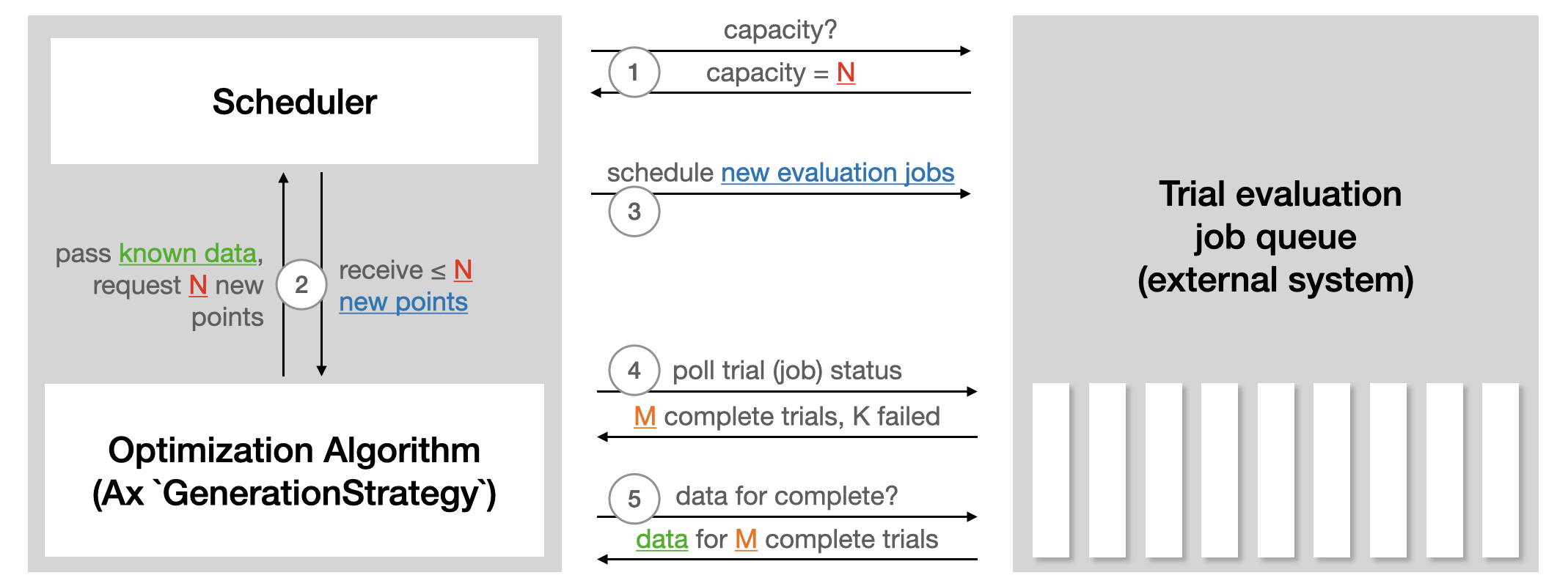
Scheduler 需要 Experiment 和 GenerationStrategy。可以通过 SchedulerOptions 提供一组选项。在这里，我们配置总评估次数以及 max_pending_trials，也就是应并行运行的试验的最大数量。在本地设置中，这是作为单独进程运行的训练任务的数量，而在远程执行设置中，这将是您希望并行使用的机器数量。

from ax.service.scheduler import Scheduler, SchedulerOptions

scheduler = Scheduler(
    experiment=experiment,
    generation_strategy=gs,
    options=SchedulerOptions(
        total_trials=total_trials, max_pending_trials=4
    ),
)

运行优化

现在，一切都已配置完毕，我们可以让 Ax 完全自动化地运行优化。Scheduler 将定期检查所有当前运行试验的状态日志，如果某个试验完成，调度器将更新实验中的状态并获取贝叶斯优化算法所需的观测值。

scheduler.run_all_trials()

评估结果

现在我们可以使用 Ax 包含的辅助函数和可视化工具来检查优化的结果。

首先，我们生成一个包含实验结果摘要的数据框。此数据框中的每一行对应一个试验（即运行的训练任务），并包含关于试验状态、评估的参数配置和观察到的度量值的信息。这提供了一种检查优化结果的便捷方式。

from ax.service.utils.report_utils import exp_to_df

df = exp_to_df(experiment)
df.head(10)

我们还可以可视化验证精度和模型参数数量之间的折衷的帕累托前沿。

小技巧

Ax 使用 Plotly 生成交互式图表，允许您进行缩放、裁剪或悬停以查看图中各部分的详细信息。您可以试试看，如果想了解更多内容，请查看 可视化教程。

最终优化结果如下图所示，其中颜色对应每次试验的迭代次数。我们看到，我们的方法成功地探索了折衷权衡，发现了既有高验证精度的大型模型，也有相对较低验证精度的小型模型。

from ax.service.utils.report_utils import _pareto_frontier_scatter_2d_plotly

_pareto_frontier_scatter_2d_plotly(experiment)

为了更好地理解我们的代理模型对黑箱目标的学习情况，我们可以查看留一交叉验证结果。由于我们的模型是高斯过程，它们不仅提供点预测，还提供了关于这些预测的不确定性估计。一个好的模型意味着预测均值（图中的点）接近 45 度线，并且置信区间以预期的频率覆盖 45 度线（这里我们使用 95% 的置信区间，因此我们预计在 95% 的情况下包含真实观测值）。

如下图所示，模型规模（num_params）度量比验证精度（val_acc）度量更容易建模。

from ax.modelbridge.cross_validation import compute_diagnostics, cross_validate
from ax.plot.diagnostic import interact_cross_validation_plotly
from ax.utils.notebook.plotting import init_notebook_plotting, render

cv = cross_validate(model=gs.model)  # The surrogate model is stored on the ``GenerationStrategy``
compute_diagnostics(cv)

interact_cross_validation_plotly(cv)

我们还可以绘制等高线图，以更好地理解不同目标如何依赖于两个输入参数。在下图中，我们显示了模型预测的验证精度作为两个隐藏层大小的函数。验证精度明显随着隐藏层大小的增大而增加。

from ax.plot.contour import interact_contour_plotly

interact_contour_plotly(model=gs.model, metric_name="val_acc")

类似地，我们在下图中显示了模型参数数量作为隐藏层大小的函数，发现其也随着隐藏层大小的增大而增加（对 hidden_size_1 的依赖性更大）。

interact_contour_plotly(model=gs.model, metric_name="num_params")

致谢

我们感谢 TorchX 团队（特别是 Kiuk Chung 和 Tristan Rice）在将 TorchX 与 Ax 集成方面的帮助。