知识蒸馏教程

Created On: Aug 22, 2023 | Last Updated: Jan 24, 2025 | Last Verified: Nov 05, 2024

作者: Alexandros Chariton

知识蒸馏是一种技术，可以将大型、计算开销高的模型的知识传递到更小的模型中，同时不失去模型的有效性。这允许在性能较低的硬件上部署，从而使评估变得更快速、更高效。

在本教程中，我们将通过一系列实验，重点提高轻量级神经网络的准确性，使用更强大的网络作为教师。轻量级网络的计算成本和速度将保持不变，我们的干预仅聚焦于其权重，而不是前向传递。这项技术的应用可以在诸如无人机或手机等设备中找到。在本教程中，我们没有使用任何外部包，因为我们所需的一切都可以在“torch”和“torchvision”中找到。

在本教程中，您将学习：

• 如何修改模型类以提取隐藏表示并将它们用于进一步计算

• 如何修改PyTorch中的常规训练循环以包括其他损失，例如用于分类的交叉熵损失之上

• 如何使用更复杂的模型作为教师来提高轻量级模型的性能

前提条件

• 1个GPU，4GB内存

• PyTorch v2.0或更高版本

• CIFAR-10数据集（由脚本下载并保存到名为“/data”的目录中）

import torch
import torch.nn as nn
import torch.optim as optim
import torchvision.transforms as transforms
import torchvision.datasets as datasets

# Check if the current `accelerator <https://pytorch.org/docs/stable/torch.html#accelerators>`__
# is available, and if not, use the CPU
device = torch.accelerator.current_accelerator().type if torch.accelerator.is_available() else "cpu"
print(f"Using {device} device")

Using cuda device

加载CIFAR-10

CIFAR-10是一个流行的包含10类图像的数据集。我们的目标是为每个输入图像预测以下类别之一。

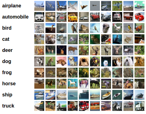
CIFAR-10图像示例

输入图像是RGB图像，因此它们有3个通道，并为32x32像素。基本上，每个图像由3 x 32 x 32 = 3072个0到255范围内的数字描述。神经网络中的一个常见做法是对输入进行归一化，这是出于多种原因，包括避免常用激活函数中的饱和现象以及提高数值稳定性。我们的归一化过程包括减去每个通道的平均值并除以标准差。张量”mean=[0.485, 0.456, 0.406]”和”std=[0.229, 0.224, 0.225]”已经计算好，它们分别表示了CIFAR-10训练集预先定义子集的每个通道的平均值和标准差。注意，我们对测试集也使用这些值，而没有从头重新计算平均值和标准差。这是因为网络是在通过减去和除以上述数值后生成的特征上训练的，我们希望保持一致性。此外，在实际中，由于我们的假设，测试集数据在那个阶段往往不可访问，因此我们无法计算其平均值和标准差。

作为一个总结的一点，我们通常将此保持出的数据集称为验证集，并在优化模型的性能时选用单独的数据集，称为测试集。这是为了避免在单一指标上的贪婪和带偏优化下选择模型。

# Below we are preprocessing data for CIFAR-10. We use an arbitrary batch size of 128.
transforms_cifar = transforms.Compose([
    transforms.ToTensor(),
    transforms.Normalize(mean=[0.485, 0.456, 0.406], std=[0.229, 0.224, 0.225]),
])

# Loading the CIFAR-10 dataset:
train_dataset = datasets.CIFAR10(root='./data', train=True, download=True, transform=transforms_cifar)
test_dataset = datasets.CIFAR10(root='./data', train=False, download=True, transform=transforms_cifar)

备注

此部分仅适用于对快速结果感兴趣的CPU用户。如果您仅对小规模实验感兴趣，可以使用此选项。请注意，使用任何GPU代码运行速度应该会相当快。只需从训练/测试数据集选择前“num_images_to_keep”图像

#from torch.utils.data import Subset
#num_images_to_keep = 2000
#train_dataset = Subset(train_dataset, range(min(num_images_to_keep, 50_000)))
#test_dataset = Subset(test_dataset, range(min(num_images_to_keep, 10_000)))

#Dataloaders
train_loader = torch.utils.data.DataLoader(train_dataset, batch_size=128, shuffle=True, num_workers=2)
test_loader = torch.utils.data.DataLoader(test_dataset, batch_size=128, shuffle=False, num_workers=2)

定义模型类和实用函数

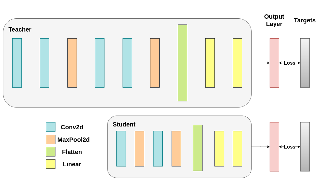
接下来，我们需要定义模型类。这里需要设置几个用户定义的参数。我们使用了两种不同的架构，在整个实验中保持滤波器数量固定以确保公平比较。两种架构都是卷积神经网络（CNN），有不同数量的卷积层作为特征提取器，随后是一个具有10个类别的分类器。学生模型的滤波器和神经元数量较少。

# Deeper neural network class to be used as teacher:
class DeepNN(nn.Module):
    def __init__(self, num_classes=10):
        super(DeepNN, self).__init__()
        self.features = nn.Sequential(
            nn.Conv2d(3, 128, kernel_size=3, padding=1),
            nn.ReLU(),
            nn.Conv2d(128, 64, kernel_size=3, padding=1),
            nn.ReLU(),
            nn.MaxPool2d(kernel_size=2, stride=2),
            nn.Conv2d(64, 64, kernel_size=3, padding=1),
            nn.ReLU(),
            nn.Conv2d(64, 32, kernel_size=3, padding=1),
            nn.ReLU(),
            nn.MaxPool2d(kernel_size=2, stride=2),
        )
        self.classifier = nn.Sequential(
            nn.Linear(2048, 512),
            nn.ReLU(),
            nn.Dropout(0.1),
            nn.Linear(512, num_classes)
        )

    def forward(self, x):
        x = self.features(x)
        x = torch.flatten(x, 1)
        x = self.classifier(x)
        return x

# Lightweight neural network class to be used as student:
class LightNN(nn.Module):
    def __init__(self, num_classes=10):
        super(LightNN, self).__init__()
        self.features = nn.Sequential(
            nn.Conv2d(3, 16, kernel_size=3, padding=1),
            nn.ReLU(),
            nn.MaxPool2d(kernel_size=2, stride=2),
            nn.Conv2d(16, 16, kernel_size=3, padding=1),
            nn.ReLU(),
            nn.MaxPool2d(kernel_size=2, stride=2),
        )
        self.classifier = nn.Sequential(
            nn.Linear(1024, 256),
            nn.ReLU(),
            nn.Dropout(0.1),
            nn.Linear(256, num_classes)
        )

    def forward(self, x):
        x = self.features(x)
        x = torch.flatten(x, 1)
        x = self.classifier(x)
        return x

我们使用2个函数来帮助我们产生和评估原始分类任务的结果。一个函数名为“train”，其参数包括：

• “model”：模型实例，通过此函数对其进行训练（更新其权重）。

• “train_loader”：我们在上面定义了“train_loader”，它的工作是将数据输入模型。

• “epochs”：循环遍历数据集的次数。

• “learning_rate”：学习率决定了我们收敛的步伐大小。步伐太大或太小都会产生负面影响。

• “device”：决定运行任务的设备。根据可用性，既可以是CPU也可以是GPU。

我们的测试函数与之类似，但会通过“test_loader”加载测试数据集的图像。

用交叉熵训练两个网络。学生网络将用作基准：

def train(model, train_loader, epochs, learning_rate, device):
    criterion = nn.CrossEntropyLoss()
    optimizer = optim.Adam(model.parameters(), lr=learning_rate)

    model.train()

    for epoch in range(epochs):
        running_loss = 0.0
        for inputs, labels in train_loader:
            # inputs: A collection of batch_size images
            # labels: A vector of dimensionality batch_size with integers denoting class of each image
            inputs, labels = inputs.to(device), labels.to(device)

            optimizer.zero_grad()
            outputs = model(inputs)

            # outputs: Output of the network for the collection of images. A tensor of dimensionality batch_size x num_classes
            # labels: The actual labels of the images. Vector of dimensionality batch_size
            loss = criterion(outputs, labels)
            loss.backward()
            optimizer.step()

            running_loss += loss.item()

        print(f"Epoch {epoch+1}/{epochs}, Loss: {running_loss / len(train_loader)}")

def test(model, test_loader, device):
    model.to(device)
    model.eval()

    correct = 0
    total = 0

    with torch.no_grad():
        for inputs, labels in test_loader:
            inputs, labels = inputs.to(device), labels.to(device)

            outputs = model(inputs)
            _, predicted = torch.max(outputs.data, 1)

            total += labels.size(0)
            correct += (predicted == labels).sum().item()

    accuracy = 100 * correct / total
    print(f"Test Accuracy: {accuracy:.2f}%")
    return accuracy

交叉熵运行

为了重现结果，我们需要设置 torch 的手动随机种子。我们使用不同的方法训练网络，因此为了公平比较，需要使用相同的权重初始化网络。首先用交叉熵训练教师网络：

torch.manual_seed(42)
nn_deep = DeepNN(num_classes=10).to(device)
train(nn_deep, train_loader, epochs=10, learning_rate=0.001, device=device)
test_accuracy_deep = test(nn_deep, test_loader, device)

# Instantiate the lightweight network:
torch.manual_seed(42)
nn_light = LightNN(num_classes=10).to(device)

Epoch 1/10, Loss: 1.3224012155057219
Epoch 2/10, Loss: 0.8630627262622804
Epoch 3/10, Loss: 0.6826653831907551
Epoch 4/10, Loss: 0.5373996891024168
Epoch 5/10, Loss: 0.41410959228072936
Epoch 6/10, Loss: 0.3109822625394367
Epoch 7/10, Loss: 0.22271543777431063
Epoch 8/10, Loss: 0.16428451289606216
Epoch 9/10, Loss: 0.14380119742868502
Epoch 10/10, Loss: 0.11495024355037896
Test Accuracy: 74.75%

我们再实例化一个轻量级网络模型以比较其性能。反向传播对权重初始化非常敏感，因此需要确保这两个网络具有完全相同的初始化。

torch.manual_seed(42)
new_nn_light = LightNN(num_classes=10).to(device)

为了确保我们已复制了第一个网络，我们检查其第一层的范数。如果匹配，则可以安全地得出结论，这两个网络确实相同。

# Print the norm of the first layer of the initial lightweight model
print("Norm of 1st layer of nn_light:", torch.norm(nn_light.features[0].weight).item())
# Print the norm of the first layer of the new lightweight model
print("Norm of 1st layer of new_nn_light:", torch.norm(new_nn_light.features[0].weight).item())

Norm of 1st layer of nn_light: 2.327361822128296
Norm of 1st layer of new_nn_light: 2.327361822128296

打印每个模型的总参数数量：

total_params_deep = "{:,}".format(sum(p.numel() for p in nn_deep.parameters()))
print(f"DeepNN parameters: {total_params_deep}")
total_params_light = "{:,}".format(sum(p.numel() for p in nn_light.parameters()))
print(f"LightNN parameters: {total_params_light}")

DeepNN parameters: 1,186,986
LightNN parameters: 267,738

用交叉熵损失训练和测试轻量级网络：

train(nn_light, train_loader, epochs=10, learning_rate=0.001, device=device)
test_accuracy_light_ce = test(nn_light, test_loader, device)

Epoch 1/10, Loss: 1.4696339499919922
Epoch 2/10, Loss: 1.1551047908070753
Epoch 3/10, Loss: 1.024265954713992
Epoch 4/10, Loss: 0.921335280246442
Epoch 5/10, Loss: 0.8481155222334216
Epoch 6/10, Loss: 0.781271718042281
Epoch 7/10, Loss: 0.71654487250711
Epoch 8/10, Loss: 0.6589792632995664
Epoch 9/10, Loss: 0.6080547195413838
Epoch 10/10, Loss: 0.5597692138093817
Test Accuracy: 70.29%

如我们所见，根据测试准确率，现在可以将作为教师的深层网络与作为假定学生的轻量级网络进行比较。目前为止，学生网络还没有干预教师，因此此性能是由学生本身实现的。到目前为止的度量可以通过以下行看到：

print(f"Teacher accuracy: {test_accuracy_deep:.2f}%")
print(f"Student accuracy: {test_accuracy_light_ce:.2f}%")

Teacher accuracy: 74.75%
Student accuracy: 70.29%

知识蒸馏运行

现在让我们尝试通过引入教师网络来提高学生网络的测试准确率。知识蒸馏是一种基于两种网络对类别输出概率分布的简单技术。因此，这两个网络共享相同数量的输出神经元。该方法通过在传统交叉熵损失中加入一个附加损失来工作，该附加损失基于教师网络的 softmax 输出。假设一个经过适当训练的教师网络的输出激活包含额外的信息，学生网络在训练过程中可以利用这些信息。原始研究表明，利用软目标中较小概率的比例可以帮助实现深度神经网络的基本目标，即在数据上创建一个相似性结构，其中相似的对象被映射得更接近。例如，在 CIFAR-10 数据集中，如果卡车带有轮子，可能会被误认为是汽车或飞机，但很少会被误认为是狗。因此，假设一个经过适当训练的模型的所有输出分布中都存在有价值的信息是有意义的，而不仅仅是其最高预测。但交叉熵并不能充分利用这些信息，因为非预测类别的激活往往过小，反向传播的梯度不能有效地改变权重以构建所期望的向量空间。

在定义第一个引入教师-学生动态的辅助函数时，我们需要包括一些额外的参数：

• T：温度控制输出分布的平滑程度。较大的 T 会导致分布更平滑，因此小概率会获得更大的提升。

• soft_target_loss_weight：分配给我们将要包含的额外目标的权重。

• ce_loss_weight：分配给交叉熵的权重。调整这些权重可引导网络优化目标。

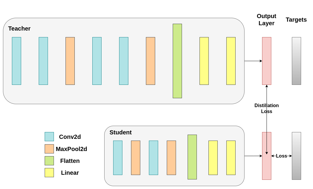
蒸馏损失根据网络的 logits 计算，仅对学生返回梯度：

def train_knowledge_distillation(teacher, student, train_loader, epochs, learning_rate, T, soft_target_loss_weight, ce_loss_weight, device):
    ce_loss = nn.CrossEntropyLoss()
    optimizer = optim.Adam(student.parameters(), lr=learning_rate)

    teacher.eval()  # Teacher set to evaluation mode
    student.train() # Student to train mode

    for epoch in range(epochs):
        running_loss = 0.0
        for inputs, labels in train_loader:
            inputs, labels = inputs.to(device), labels.to(device)

            optimizer.zero_grad()

            # Forward pass with the teacher model - do not save gradients here as we do not change the teacher's weights
            with torch.no_grad():
                teacher_logits = teacher(inputs)

            # Forward pass with the student model
            student_logits = student(inputs)

            #Soften the student logits by applying softmax first and log() second
            soft_targets = nn.functional.softmax(teacher_logits / T, dim=-1)
            soft_prob = nn.functional.log_softmax(student_logits / T, dim=-1)

            # Calculate the soft targets loss. Scaled by T**2 as suggested by the authors of the paper "Distilling the knowledge in a neural network"
            soft_targets_loss = torch.sum(soft_targets * (soft_targets.log() - soft_prob)) / soft_prob.size()[0] * (T**2)

            # Calculate the true label loss
            label_loss = ce_loss(student_logits, labels)

            # Weighted sum of the two losses
            loss = soft_target_loss_weight * soft_targets_loss + ce_loss_weight * label_loss

            loss.backward()
            optimizer.step()

            running_loss += loss.item()

        print(f"Epoch {epoch+1}/{epochs}, Loss: {running_loss / len(train_loader)}")

# Apply ``train_knowledge_distillation`` with a temperature of 2. Arbitrarily set the weights to 0.75 for CE and 0.25 for distillation loss.
train_knowledge_distillation(teacher=nn_deep, student=new_nn_light, train_loader=train_loader, epochs=10, learning_rate=0.001, T=2, soft_target_loss_weight=0.25, ce_loss_weight=0.75, device=device)
test_accuracy_light_ce_and_kd = test(new_nn_light, test_loader, device)

# Compare the student test accuracy with and without the teacher, after distillation
print(f"Teacher accuracy: {test_accuracy_deep:.2f}%")
print(f"Student accuracy without teacher: {test_accuracy_light_ce:.2f}%")
print(f"Student accuracy with CE + KD: {test_accuracy_light_ce_and_kd:.2f}%")

Epoch 1/10, Loss: 2.378872389378755
Epoch 2/10, Loss: 1.8624892204313936
Epoch 3/10, Loss: 1.6402246680710932
Epoch 4/10, Loss: 1.4804699536784531
Epoch 5/10, Loss: 1.3535917960774257
Epoch 6/10, Loss: 1.237514083647667
Epoch 7/10, Loss: 1.1402380141760686
Epoch 8/10, Loss: 1.0539719300806676
Epoch 9/10, Loss: 0.9768481629583842
Epoch 10/10, Loss: 0.909109282066755
Test Accuracy: 70.88%
Teacher accuracy: 74.75%
Student accuracy without teacher: 70.29%
Student accuracy with CE + KD: 70.88%

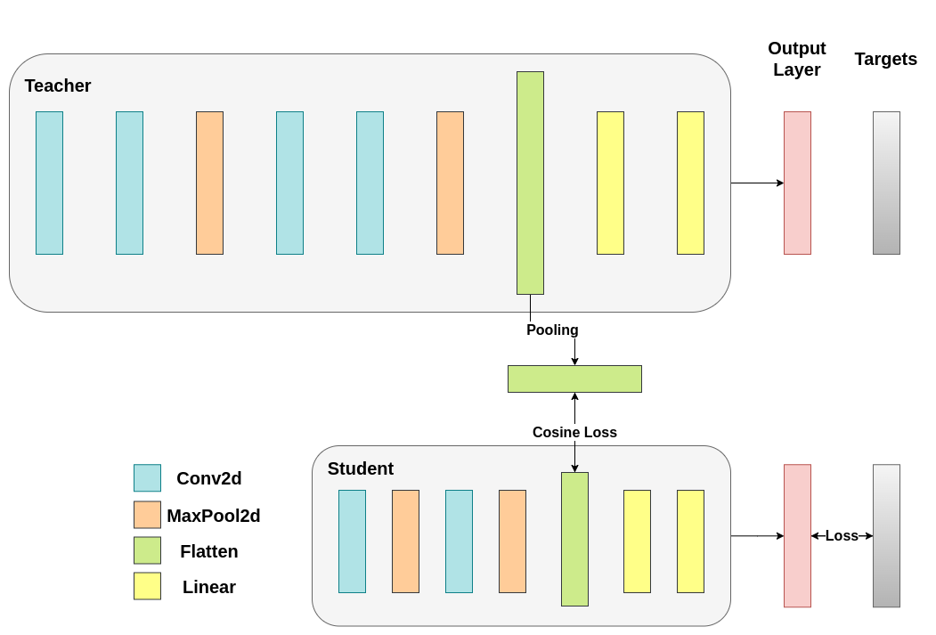
余弦损失最小化运行

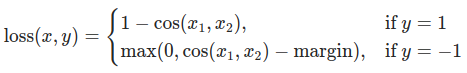
可以自由调整控制 softmax 函数柔和程度的温度参数和损失系数。在神经网络中，通过在主要目标中加入额外的损失函数，可以实现更好的泛化效果。让我们尝试为学生包含一个目标，但这次聚焦于隐藏层状态而不是输出层。我们的目标是通过包括一个简单的损失函数，使得被分类器随后传递的展平向量随着损失的减少变得更加 相似。当然，教师不会更新其权重，因此最小化仅取决于学生的权重。此方法的基本原理是我们假设教师模型具有更好的内部表示，学生在没有外部干预的情况下不可能达到，因此我们人为地推动学生模仿教师的内部表示。然而，这是否有助于学生并不直观，因为推动轻量级网络到达此状态可能是好事，假设我们确实找到了一个导致更优测试准确率的内部表示，但也可能有害，因为网络具有不同的架构，学生的学习能力不同于教师。换句话说，没有理由要求这两个向量，学生的和教师的，在每个分量上都匹配。学生可以达到一个是教师表示的置换的内部表示，这同样高效。不过，我们仍然可以运行一个快速实验来了解此方法的影响。我们将使用``CosineEmbeddingLoss``，其公式如下：

CosineEmbeddingLoss公式

显然，我们需要先解决一个问题。当我们在输出层应用蒸馏时提到，两种网络拥有相同数量的神经元，等于类别数。然而，这并不适用于卷积层之后的层次。这里，教师在最终卷积层展平后的神经元数多于学生。我们的损失函数接受两个具有相同维数的向量作为输入，因此我们需要以某种方式匹配它们。我们将通过在教师的卷积层之后包括一个平均池化层来解决这个问题，该层将其维数缩小，以与学生匹配。

接下来，我们将修改模型类，或者创建新类。现在，前向函数不仅返回网络的 logits，还返回卷积层后的展平隐藏表示。对于修改后的教师网络，我们包括上述池化操作。

class ModifiedDeepNNCosine(nn.Module):
    def __init__(self, num_classes=10):
        super(ModifiedDeepNNCosine, self).__init__()
        self.features = nn.Sequential(
            nn.Conv2d(3, 128, kernel_size=3, padding=1),
            nn.ReLU(),
            nn.Conv2d(128, 64, kernel_size=3, padding=1),
            nn.ReLU(),
            nn.MaxPool2d(kernel_size=2, stride=2),
            nn.Conv2d(64, 64, kernel_size=3, padding=1),
            nn.ReLU(),
            nn.Conv2d(64, 32, kernel_size=3, padding=1),
            nn.ReLU(),
            nn.MaxPool2d(kernel_size=2, stride=2),
        )
        self.classifier = nn.Sequential(
            nn.Linear(2048, 512),
            nn.ReLU(),
            nn.Dropout(0.1),
            nn.Linear(512, num_classes)
        )

    def forward(self, x):
        x = self.features(x)
        flattened_conv_output = torch.flatten(x, 1)
        x = self.classifier(flattened_conv_output)
        flattened_conv_output_after_pooling = torch.nn.functional.avg_pool1d(flattened_conv_output, 2)
        return x, flattened_conv_output_after_pooling

# Create a similar student class where we return a tuple. We do not apply pooling after flattening.
class ModifiedLightNNCosine(nn.Module):
    def __init__(self, num_classes=10):
        super(ModifiedLightNNCosine, self).__init__()
        self.features = nn.Sequential(
            nn.Conv2d(3, 16, kernel_size=3, padding=1),
            nn.ReLU(),
            nn.MaxPool2d(kernel_size=2, stride=2),
            nn.Conv2d(16, 16, kernel_size=3, padding=1),
            nn.ReLU(),
            nn.MaxPool2d(kernel_size=2, stride=2),
        )
        self.classifier = nn.Sequential(
            nn.Linear(1024, 256),
            nn.ReLU(),
            nn.Dropout(0.1),
            nn.Linear(256, num_classes)
        )

    def forward(self, x):
        x = self.features(x)
        flattened_conv_output = torch.flatten(x, 1)
        x = self.classifier(flattened_conv_output)
        return x, flattened_conv_output

# We do not have to train the modified deep network from scratch of course, we just load its weights from the trained instance
modified_nn_deep = ModifiedDeepNNCosine(num_classes=10).to(device)
modified_nn_deep.load_state_dict(nn_deep.state_dict())

# Once again ensure the norm of the first layer is the same for both networks
print("Norm of 1st layer for deep_nn:", torch.norm(nn_deep.features[0].weight).item())
print("Norm of 1st layer for modified_deep_nn:", torch.norm(modified_nn_deep.features[0].weight).item())

# Initialize a modified lightweight network with the same seed as our other lightweight instances. This will be trained from scratch to examine the effectiveness of cosine loss minimization.
torch.manual_seed(42)
modified_nn_light = ModifiedLightNNCosine(num_classes=10).to(device)
print("Norm of 1st layer:", torch.norm(modified_nn_light.features[0].weight).item())

Norm of 1st layer for deep_nn: 7.503961086273193
Norm of 1st layer for modified_deep_nn: 7.503961086273193
Norm of 1st layer: 2.327361822128296

自然地，我们需要更改训练循环，因为现在模型返回一个元组``(logits, hidden_representation)``。使用一个示例输入张量，我们可以打印其形状。

# Create a sample input tensor
sample_input = torch.randn(128, 3, 32, 32).to(device) # Batch size: 128, Filters: 3, Image size: 32x32

# Pass the input through the student
logits, hidden_representation = modified_nn_light(sample_input)

# Print the shapes of the tensors
print("Student logits shape:", logits.shape) # batch_size x total_classes
print("Student hidden representation shape:", hidden_representation.shape) # batch_size x hidden_representation_size

# Pass the input through the teacher
logits, hidden_representation = modified_nn_deep(sample_input)

# Print the shapes of the tensors
print("Teacher logits shape:", logits.shape) # batch_size x total_classes
print("Teacher hidden representation shape:", hidden_representation.shape) # batch_size x hidden_representation_size

Student logits shape: torch.Size([128, 10])
Student hidden representation shape: torch.Size([128, 1024])
Teacher logits shape: torch.Size([128, 10])
Teacher hidden representation shape: torch.Size([128, 1024])

在我们的案例中，hidden_representation_size 是 1024。这是学生最终卷积层展平的特征图，如您所见，它是其分类器的输入。对于教师也是``1024``，因为我们通过``avg_pool1d``从``2048``调整而来。此处应用的损失仅影响学生的权重，而不影响分类器。以下是修改后的训练循环：

在余弦损失最小化中，我们希望通过将梯度返回给学生来最大化两个表示的余弦相似度：

def train_cosine_loss(teacher, student, train_loader, epochs, learning_rate, hidden_rep_loss_weight, ce_loss_weight, device):
    ce_loss = nn.CrossEntropyLoss()
    cosine_loss = nn.CosineEmbeddingLoss()
    optimizer = optim.Adam(student.parameters(), lr=learning_rate)

    teacher.to(device)
    student.to(device)
    teacher.eval()  # Teacher set to evaluation mode
    student.train() # Student to train mode

    for epoch in range(epochs):
        running_loss = 0.0
        for inputs, labels in train_loader:
            inputs, labels = inputs.to(device), labels.to(device)

            optimizer.zero_grad()

            # Forward pass with the teacher model and keep only the hidden representation
            with torch.no_grad():
                _, teacher_hidden_representation = teacher(inputs)

            # Forward pass with the student model
            student_logits, student_hidden_representation = student(inputs)

            # Calculate the cosine loss. Target is a vector of ones. From the loss formula above we can see that is the case where loss minimization leads to cosine similarity increase.
            hidden_rep_loss = cosine_loss(student_hidden_representation, teacher_hidden_representation, target=torch.ones(inputs.size(0)).to(device))

            # Calculate the true label loss
            label_loss = ce_loss(student_logits, labels)

            # Weighted sum of the two losses
            loss = hidden_rep_loss_weight * hidden_rep_loss + ce_loss_weight * label_loss

            loss.backward()
            optimizer.step()

            running_loss += loss.item()

        print(f"Epoch {epoch+1}/{epochs}, Loss: {running_loss / len(train_loader)}")

出于相同的原因，我们需要修改测试函数。这里我们忽略模型返回的隐藏表示。

def test_multiple_outputs(model, test_loader, device):
    model.to(device)
    model.eval()

    correct = 0
    total = 0

    with torch.no_grad():
        for inputs, labels in test_loader:
            inputs, labels = inputs.to(device), labels.to(device)

            outputs, _ = model(inputs) # Disregard the second tensor of the tuple
            _, predicted = torch.max(outputs.data, 1)

            total += labels.size(0)
            correct += (predicted == labels).sum().item()

    accuracy = 100 * correct / total
    print(f"Test Accuracy: {accuracy:.2f}%")
    return accuracy

在这种情况下，我们可以轻松地将知识蒸馏和余弦损失最小化包含在同一个函数中。在教师-学生范式中，组合方法以获得更好的性能是很常见的。目前，我们可以运行一个简单的训练-测试会话。

# Train and test the lightweight network with cross entropy loss
train_cosine_loss(teacher=modified_nn_deep, student=modified_nn_light, train_loader=train_loader, epochs=10, learning_rate=0.001, hidden_rep_loss_weight=0.25, ce_loss_weight=0.75, device=device)
test_accuracy_light_ce_and_cosine_loss = test_multiple_outputs(modified_nn_light, test_loader, device)

Epoch 1/10, Loss: 1.3018172540323203
Epoch 2/10, Loss: 1.0700001532159498
Epoch 3/10, Loss: 0.9706814766235059
Epoch 4/10, Loss: 0.8953244106848831
Epoch 5/10, Loss: 0.8393775093585939
Epoch 6/10, Loss: 0.7944566558693986
Epoch 7/10, Loss: 0.7529576269866866
Epoch 8/10, Loss: 0.7171070446138796
Epoch 9/10, Loss: 0.6798297279631086
Epoch 10/10, Loss: 0.6551050700799889
Test Accuracy: 70.44%

中间回归器运行

我们的简单最小化不能保证更好的结果，其中一个原因是向量的维数。余弦相似性通常比欧几里得距离在高维向量上更有效，但我们处理的是每个拥有 1024 个组成部分的向量，因此难以提取有意义的相似性。此外，如我们提到的，推动教师和学生的隐藏表示匹配在理论上并不支持。没有充分的理由认为我们应该追求这些向量的 1:1 匹配。我们将通过包含一个称为回归器的额外网络来提供一个最终的训练干预示例。目标是首先提取教师在卷积层后的特征图，然后提取学生在卷积层后的特征图，最后尝试匹配这些特征图。然而，这一次，我们将在网络之间引入一个回归器来促进匹配过程。回归器是可训练的，理想情况下会比我们简单的余弦损失最小化方案表现更好。其主要任务是匹配这些特征图的维数，以便我们可以在教师和学生之间正确定义损失函数。定义这样的损失函数提供了一条“教学路径”，即反向传播梯度的流，以更改学生的权重。聚焦于分类器之前每个网络的卷积层输出，我们有以下形状：

# Pass the sample input only from the convolutional feature extractor
convolutional_fe_output_student = nn_light.features(sample_input)
convolutional_fe_output_teacher = nn_deep.features(sample_input)

# Print their shapes
print("Student's feature extractor output shape: ", convolutional_fe_output_student.shape)
print("Teacher's feature extractor output shape: ", convolutional_fe_output_teacher.shape)

Student's feature extractor output shape:  torch.Size([128, 16, 8, 8])
Teacher's feature extractor output shape:  torch.Size([128, 32, 8, 8])

教师网络有 32 个滤波器，学生网络有 16 个滤波器。我们将在学生特征图和教师特征图之间加入一个可训练的层，转换学生的特征图形状以匹配教师的特征图形状。在实践中，我们修改轻量级类别，使其返回经过中间回归器后的隐藏状态，这些回归器匹配卷积特征图的尺寸，并修改教师类别以返回最终卷积层的输出（不进行池化或展平）。

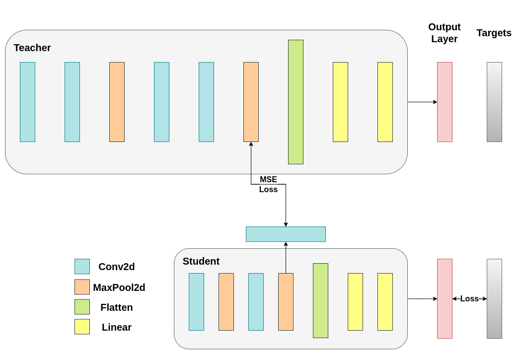
该可训练层匹配中间张量的形状，均方误差 (MSE) 可正确定义：

class ModifiedDeepNNRegressor(nn.Module):
    def __init__(self, num_classes=10):
        super(ModifiedDeepNNRegressor, self).__init__()
        self.features = nn.Sequential(
            nn.Conv2d(3, 128, kernel_size=3, padding=1),
            nn.ReLU(),
            nn.Conv2d(128, 64, kernel_size=3, padding=1),
            nn.ReLU(),
            nn.MaxPool2d(kernel_size=2, stride=2),
            nn.Conv2d(64, 64, kernel_size=3, padding=1),
            nn.ReLU(),
            nn.Conv2d(64, 32, kernel_size=3, padding=1),
            nn.ReLU(),
            nn.MaxPool2d(kernel_size=2, stride=2),
        )
        self.classifier = nn.Sequential(
            nn.Linear(2048, 512),
            nn.ReLU(),
            nn.Dropout(0.1),
            nn.Linear(512, num_classes)
        )

    def forward(self, x):
        x = self.features(x)
        conv_feature_map = x
        x = torch.flatten(x, 1)
        x = self.classifier(x)
        return x, conv_feature_map

class ModifiedLightNNRegressor(nn.Module):
    def __init__(self, num_classes=10):
        super(ModifiedLightNNRegressor, self).__init__()
        self.features = nn.Sequential(
            nn.Conv2d(3, 16, kernel_size=3, padding=1),
            nn.ReLU(),
            nn.MaxPool2d(kernel_size=2, stride=2),
            nn.Conv2d(16, 16, kernel_size=3, padding=1),
            nn.ReLU(),
            nn.MaxPool2d(kernel_size=2, stride=2),
        )
        # Include an extra regressor (in our case linear)
        self.regressor = nn.Sequential(
            nn.Conv2d(16, 32, kernel_size=3, padding=1)
        )
        self.classifier = nn.Sequential(
            nn.Linear(1024, 256),
            nn.ReLU(),
            nn.Dropout(0.1),
            nn.Linear(256, num_classes)
        )

    def forward(self, x):
        x = self.features(x)
        regressor_output = self.regressor(x)
        x = torch.flatten(x, 1)
        x = self.classifier(x)
        return x, regressor_output

之后，我们需要再次更新训练循环。这次，我们提取学生的回归器输出和教师的特征图，在这些具有相同形状的张量上计算 MSE，然后基于该损失以及分类任务的常规交叉熵损失进行反向传播梯度。

def train_mse_loss(teacher, student, train_loader, epochs, learning_rate, feature_map_weight, ce_loss_weight, device):
    ce_loss = nn.CrossEntropyLoss()
    mse_loss = nn.MSELoss()
    optimizer = optim.Adam(student.parameters(), lr=learning_rate)

    teacher.to(device)
    student.to(device)
    teacher.eval()  # Teacher set to evaluation mode
    student.train() # Student to train mode

    for epoch in range(epochs):
        running_loss = 0.0
        for inputs, labels in train_loader:
            inputs, labels = inputs.to(device), labels.to(device)

            optimizer.zero_grad()

            # Again ignore teacher logits
            with torch.no_grad():
                _, teacher_feature_map = teacher(inputs)

            # Forward pass with the student model
            student_logits, regressor_feature_map = student(inputs)

            # Calculate the loss
            hidden_rep_loss = mse_loss(regressor_feature_map, teacher_feature_map)

            # Calculate the true label loss
            label_loss = ce_loss(student_logits, labels)

            # Weighted sum of the two losses
            loss = feature_map_weight * hidden_rep_loss + ce_loss_weight * label_loss

            loss.backward()
            optimizer.step()

            running_loss += loss.item()

        print(f"Epoch {epoch+1}/{epochs}, Loss: {running_loss / len(train_loader)}")

# Notice how our test function remains the same here with the one we used in our previous case. We only care about the actual outputs because we measure accuracy.

# Initialize a ModifiedLightNNRegressor
torch.manual_seed(42)
modified_nn_light_reg = ModifiedLightNNRegressor(num_classes=10).to(device)

# We do not have to train the modified deep network from scratch of course, we just load its weights from the trained instance
modified_nn_deep_reg = ModifiedDeepNNRegressor(num_classes=10).to(device)
modified_nn_deep_reg.load_state_dict(nn_deep.state_dict())

# Train and test once again
train_mse_loss(teacher=modified_nn_deep_reg, student=modified_nn_light_reg, train_loader=train_loader, epochs=10, learning_rate=0.001, feature_map_weight=0.25, ce_loss_weight=0.75, device=device)
test_accuracy_light_ce_and_mse_loss = test_multiple_outputs(modified_nn_light_reg, test_loader, device)

Epoch 1/10, Loss: 1.6874313952063051
Epoch 2/10, Loss: 1.3130229235914967
Epoch 3/10, Loss: 1.1716968121431064
Epoch 4/10, Loss: 1.075458403895883
Epoch 5/10, Loss: 0.9987687174316562
Epoch 6/10, Loss: 0.9354991790888559
Epoch 7/10, Loss: 0.8837388240162979
Epoch 8/10, Loss: 0.8350984573059375
Epoch 9/10, Loss: 0.793205637151323
Epoch 10/10, Loss: 0.7540451352248716
Test Accuracy: 70.99%

我们预计最终的方法会比 CosineLoss 更好，因为现在我们允许在教师和学生之间有一个可训练层，这为学生提供了在学习时的灵活性，而不是单纯地让学生复制教师的表示。引入额外的网络层是基于提示蒸馏的理念。

print(f"Teacher accuracy: {test_accuracy_deep:.2f}%")
print(f"Student accuracy without teacher: {test_accuracy_light_ce:.2f}%")
print(f"Student accuracy with CE + KD: {test_accuracy_light_ce_and_kd:.2f}%")
print(f"Student accuracy with CE + CosineLoss: {test_accuracy_light_ce_and_cosine_loss:.2f}%")
print(f"Student accuracy with CE + RegressorMSE: {test_accuracy_light_ce_and_mse_loss:.2f}%")

Teacher accuracy: 74.75%
Student accuracy without teacher: 70.29%
Student accuracy with CE + KD: 70.88%
Student accuracy with CE + CosineLoss: 70.44%
Student accuracy with CE + RegressorMSE: 70.99%

总结

以上方法均没有增加网络参数数量或推理时间，因此性能的提升只需要在训练期间计算梯度的少量开销。在机器学习应用中，我们主要关注的是推理时间，因为训练是在模型部署之前完成的。如果我们的轻量化模型在部署时仍然太重，我们可以采用诸如训练后量化的其他方案。额外的损失函数可以应用于许多任务，而不仅限于分类问题，您可以尝试不同的值，比如系数、温度或神经元数量。随意调整上述教程中的任何数字，但请记住，如果更改神经元/过滤器的数量，很可能会出现形状不匹配的问题。

有关更多信息，请参见：

• Hinton, G., Vinyals, O., Dean, J.: Distilling the knowledge in a neural network. In: Neural Information Processing System Deep Learning Workshop (2015)

• Romero, A., Ballas, N., Kahou, S.E., Chassang, A., Gatta, C., Bengio, Y.: Fitnets: Hints for thin deep nets. In: Proceedings of the International Conference on Learning Representations (2015)