使用 TensorBoard 可视化模型、数据和训练过程

Created On: Aug 08, 2019 | Last Updated: Oct 18, 2022 | Last Verified: Nov 05, 2024

在 60 分钟入门教程 中，我们讲解了如何加载数据，将数据传入我们定义为 nn.Module 子类的模型，在训练数据上训练模型，并在测试数据上测试模型。为了观察训练过程，我们打印了模型训练时的一些统计信息，但我们可以做得更好：PyTorch 集成了 TensorBoard，一个为可视化神经网络训练结果而设计的工具。本教程将展示其一些功能，使用 Fashion-MNIST 数据集，该数据集可以通过 torchvision.datasets 加载到 PyTorch 中。

在本教程中，我们将学习如何：

1. 读取并转换数据（与前面的教程几乎相同）。

2. 设置 TensorBoard。

3. 写入数据到 TensorBoard。

4. 使用 TensorBoard 检查模型结构。

5. 使用 TensorBoard 创建前教程可视化的交互式版本，同时减少代码量。

特别是在第5点中，我们将看到：

• 几种检查训练数据的方法

• 如何跟踪模型在训练过程中的性能

• 如何评估训练后的模型性能。

我们将从类似于 CIFAR-10 教程 的基础代码开始：

# imports
import matplotlib.pyplot as plt
import numpy as np

import torch
import torchvision
import torchvision.transforms as transforms

import torch.nn as nn
import torch.nn.functional as F
import torch.optim as optim

# transforms
transform = transforms.Compose(
    [transforms.ToTensor(),
    transforms.Normalize((0.5,), (0.5,))])

# datasets
trainset = torchvision.datasets.FashionMNIST('./data',
    download=True,
    train=True,
    transform=transform)
testset = torchvision.datasets.FashionMNIST('./data',
    download=True,
    train=False,
    transform=transform)

# dataloaders
trainloader = torch.utils.data.DataLoader(trainset, batch_size=4,
                                        shuffle=True, num_workers=2)


testloader = torch.utils.data.DataLoader(testset, batch_size=4,
                                        shuffle=False, num_workers=2)

# constant for classes
classes = ('T-shirt/top', 'Trouser', 'Pullover', 'Dress', 'Coat',
        'Sandal', 'Shirt', 'Sneaker', 'Bag', 'Ankle Boot')

# helper function to show an image
# (used in the `plot_classes_preds` function below)
def matplotlib_imshow(img, one_channel=False):
    if one_channel:
        img = img.mean(dim=0)
    img = img / 2 + 0.5     # unnormalize
    npimg = img.numpy()
    if one_channel:
        plt.imshow(npimg, cmap="Greys")
    else:
        plt.imshow(np.transpose(npimg, (1, 2, 0)))

我们将定义与该教程中类似的模型架构，仅做出一些轻微修改以适应图像现在是单通道而不是三通道且大小为28x28而不是32x32的情况：

class Net(nn.Module):
    def __init__(self):
        super(Net, self).__init__()
        self.conv1 = nn.Conv2d(1, 6, 5)
        self.pool = nn.MaxPool2d(2, 2)
        self.conv2 = nn.Conv2d(6, 16, 5)
        self.fc1 = nn.Linear(16 * 4 * 4, 120)
        self.fc2 = nn.Linear(120, 84)
        self.fc3 = nn.Linear(84, 10)

    def forward(self, x):
        x = self.pool(F.relu(self.conv1(x)))
        x = self.pool(F.relu(self.conv2(x)))
        x = x.view(-1, 16 * 4 * 4)
        x = F.relu(self.fc1(x))
        x = F.relu(self.fc2(x))
        x = self.fc3(x)
        return x


net = Net()

我们将定义与之前相同的 optimizer 和 criterion：

criterion = nn.CrossEntropyLoss()
optimizer = optim.SGD(net.parameters(), lr=0.001, momentum=0.9)

1. TensorBoard 设置

现在我们将设置 TensorBoard，从 torch.utils 导入 tensorboard 并定义一个 SummaryWriter，这是我们写入 TensorBoard 的关键对象。

from torch.utils.tensorboard import SummaryWriter

# default `log_dir` is "runs" - we'll be more specific here
writer = SummaryWriter('runs/fashion_mnist_experiment_1')

请注意，仅这一行代码就创建了一个 runs/fashion_mnist_experiment_1 文件夹。

2. 写入数据到 TensorBoard

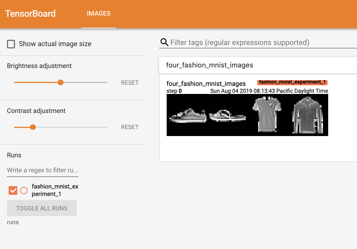
现在让我们向 TensorBoard 写入一个图像 - 确切来说是一个网格 - 使用 make_grid。

# get some random training images
dataiter = iter(trainloader)
images, labels = next(dataiter)

# create grid of images
img_grid = torchvision.utils.make_grid(images)

# show images
matplotlib_imshow(img_grid, one_channel=True)

# write to tensorboard
writer.add_image('four_fashion_mnist_images', img_grid)

现在运行

tensorboard --logdir=runs

从命令行导航到 http://localhost:6006，应该能看到以下内容。

现在您已经知道如何使用 TensorBoard！然而，这个例子可以在 Jupyter Notebook 中完成 - TensorBoard 的真正优秀之处在于创建交互式可视化。接下来我们将在教程结束前介绍一个这样的例子。

3. 使用 TensorBoard 检查模型

TensorBoard 的一个优势是能够可视化复杂的模型结构。我们来可视化我们构建的模型。

writer.add_graph(net, images)
writer.close()

刷新 TensorBoard 后，您应该能看到一个 “Graphs” 标签页，如下图所示：

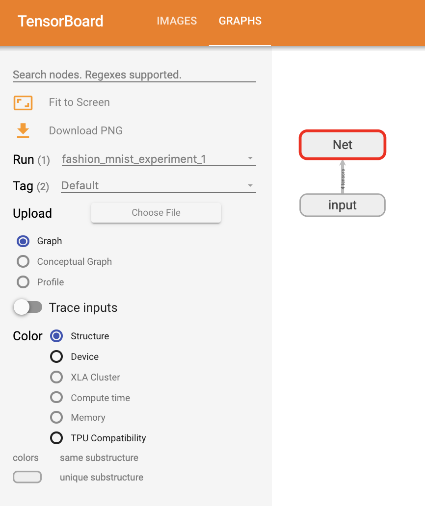
继续双击 “Net”，可以展开它，查看组成模型的各个操作的详细视图。

TensorBoard 对于将高维数据（如图像数据）可视化为低维空间非常有用；接下来我们将介绍这一功能。

4. 为 TensorBoard 添加 “Projector”

我们可以通过 add_embedding 方法可视化高维数据的低维表示。

# helper function
def select_n_random(data, labels, n=100):
    '''
    Selects n random datapoints and their corresponding labels from a dataset
    '''
    assert len(data) == len(labels)

    perm = torch.randperm(len(data))
    return data[perm][:n], labels[perm][:n]

# select random images and their target indices
images, labels = select_n_random(trainset.data, trainset.targets)

# get the class labels for each image
class_labels = [classes[lab] for lab in labels]

# log embeddings
features = images.view(-1, 28 * 28)
writer.add_embedding(features,
                    metadata=class_labels,
                    label_img=images.unsqueeze(1))
writer.close()

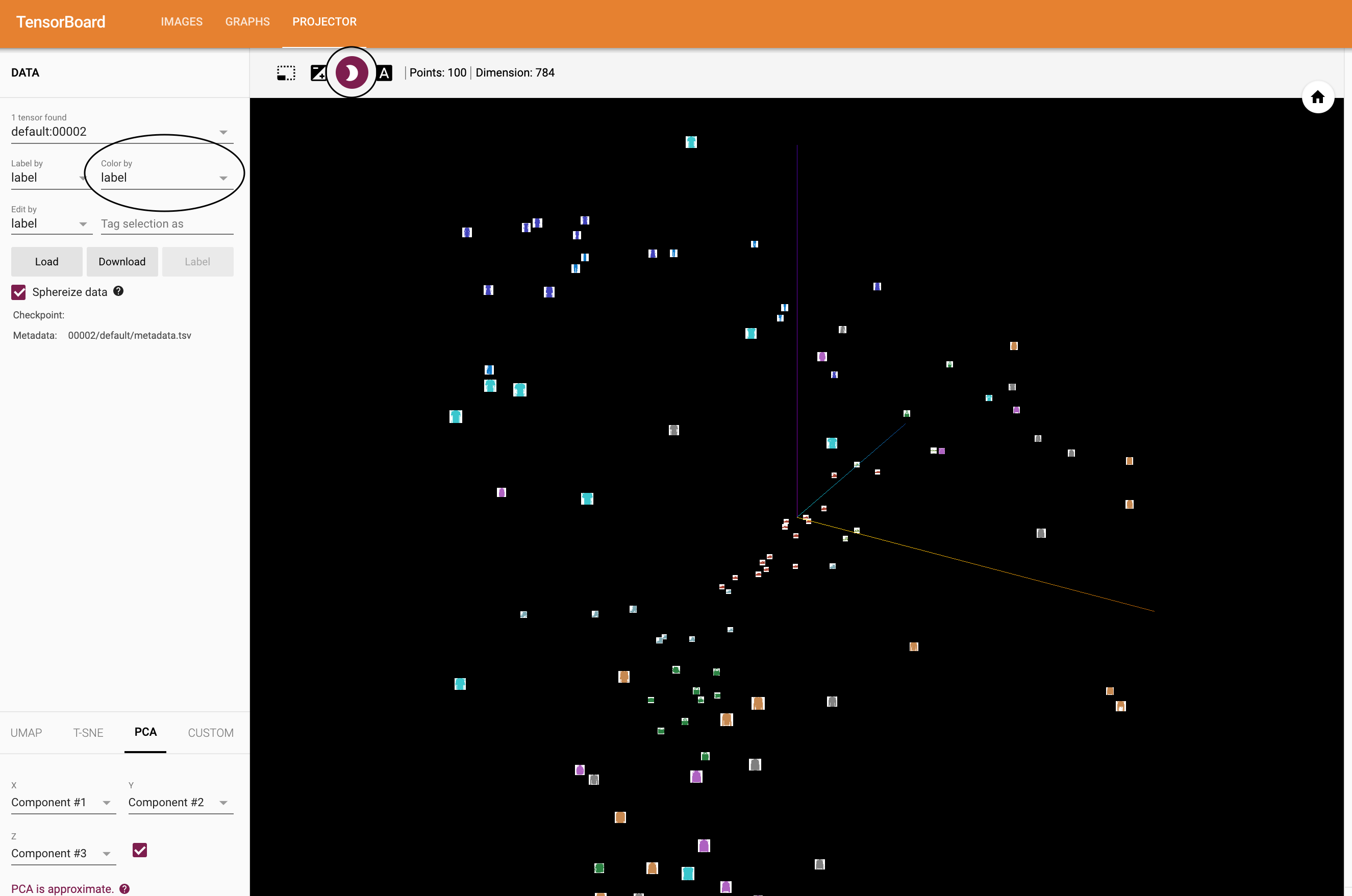
现在在 TensorBoard 的 “Projector” 标签页中，您可以看到这些100张图像 - 每张图像是784维 - 投射到三维空间中。此外，这是可交互的：您可以点击并拖曳来旋转三维投影。最后，有两个小技巧可以让可视化更容易观察：在左上角选择 “color: label”，并启用 “夜间模式”，这样图像会更容易看清，因为它们的背景是白色的：

现在我们已对数据进行了深入检查，接下来我们将展示 TensorBoard 如何使模型训练和评估的跟踪更加清晰，从训练开始。

5. 使用 TensorBoard 跟踪模型训练

在之前的例子中，我们每2000次迭代通过 print 输出模型的运行损失。现在，我们将通过 plot_classes_preds 函数将运行损失记录到 TensorBoard，同时查看模型做出的预测。

# helper functions

def images_to_probs(net, images):
    '''
    Generates predictions and corresponding probabilities from a trained
    network and a list of images
    '''
    output = net(images)
    # convert output probabilities to predicted class
    _, preds_tensor = torch.max(output, 1)
    preds = np.squeeze(preds_tensor.numpy())
    return preds, [F.softmax(el, dim=0)[i].item() for i, el in zip(preds, output)]


def plot_classes_preds(net, images, labels):
    '''
    Generates matplotlib Figure using a trained network, along with images
    and labels from a batch, that shows the network's top prediction along
    with its probability, alongside the actual label, coloring this
    information based on whether the prediction was correct or not.
    Uses the "images_to_probs" function.
    '''
    preds, probs = images_to_probs(net, images)
    # plot the images in the batch, along with predicted and true labels
    fig = plt.figure(figsize=(12, 48))
    for idx in np.arange(4):
        ax = fig.add_subplot(1, 4, idx+1, xticks=[], yticks=[])
        matplotlib_imshow(images[idx], one_channel=True)
        ax.set_title("{0}, {1:.1f}%\n(label: {2})".format(
            classes[preds[idx]],
            probs[idx] * 100.0,
            classes[labels[idx]]),
                    color=("green" if preds[idx]==labels[idx].item() else "red"))
    return fig

最后，使用前教程中的同样模型训练代码，但将每1000批次的结果写入 TensorBoard，而不是打印到控制台；这通过使用 add_scalar 函数完成。

此外，在训练过程中，我们将生成一个图像，显示模型的预测与该批次中包含的四张图像的实际结果的比较。

running_loss = 0.0
for epoch in range(1):  # loop over the dataset multiple times

    for i, data in enumerate(trainloader, 0):

        # get the inputs; data is a list of [inputs, labels]
        inputs, labels = data

        # zero the parameter gradients
        optimizer.zero_grad()

        # forward + backward + optimize
        outputs = net(inputs)
        loss = criterion(outputs, labels)
        loss.backward()
        optimizer.step()

        running_loss += loss.item()
        if i % 1000 == 999:    # every 1000 mini-batches...

            # ...log the running loss
            writer.add_scalar('training loss',
                            running_loss / 1000,
                            epoch * len(trainloader) + i)

            # ...log a Matplotlib Figure showing the model's predictions on a
            # random mini-batch
            writer.add_figure('predictions vs. actuals',
                            plot_classes_preds(net, inputs, labels),
                            global_step=epoch * len(trainloader) + i)
            running_loss = 0.0
print('Finished Training')

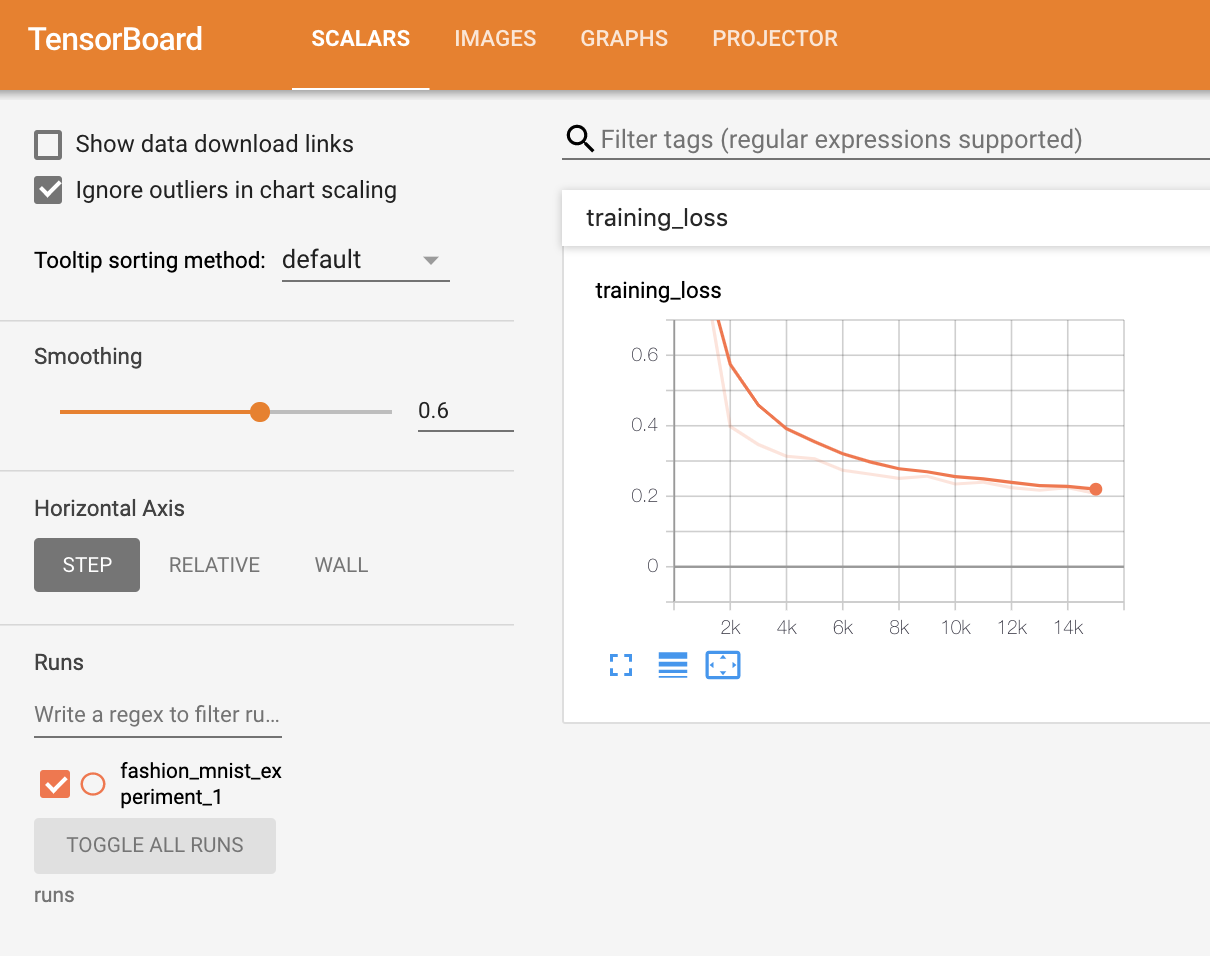
您现在可以查看标量标签页，看到持续损失在15000次迭代中的绘制：

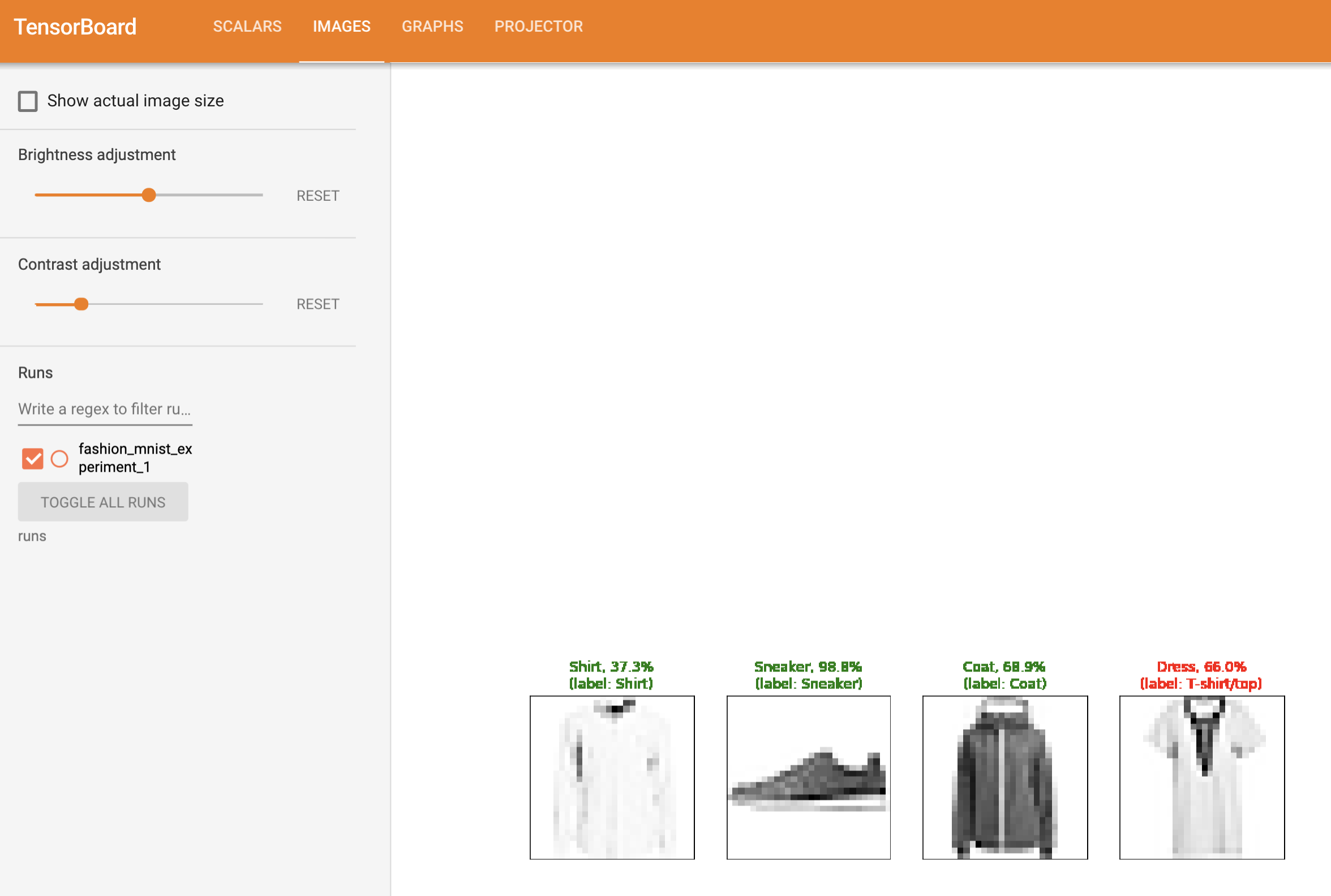
此外，我们可以查看模型在整个学习过程中对任意批次的预测。查看 “Images” 标签页，并向下滚动到 “predictions vs. actuals” 可视化以查看这一点；例如，在仅训练3000次迭代后，模型已能够区分视觉上明显不同的类别，如衬衫、运动鞋和外套，虽然它在训练后期更有信心：

在之前的教程中，我们在模型训练完成后查看了每个类别的准确率；在这里，我们将使用 TensorBoard 来绘制每个类别的精确率-召回率曲线（关于此主题的优秀解释见 这里）。

6. 使用 TensorBoard 评估训练过的模型

# 1. gets the probability predictions in a test_size x num_classes Tensor
# 2. gets the preds in a test_size Tensor
# takes ~10 seconds to run
class_probs = []
class_label = []
with torch.no_grad():
    for data in testloader:
        images, labels = data
        output = net(images)
        class_probs_batch = [F.softmax(el, dim=0) for el in output]

        class_probs.append(class_probs_batch)
        class_label.append(labels)

test_probs = torch.cat([torch.stack(batch) for batch in class_probs])
test_label = torch.cat(class_label)

# helper function
def add_pr_curve_tensorboard(class_index, test_probs, test_label, global_step=0):
    '''
    Takes in a "class_index" from 0 to 9 and plots the corresponding
    precision-recall curve
    '''
    tensorboard_truth = test_label == class_index
    tensorboard_probs = test_probs[:, class_index]

    writer.add_pr_curve(classes[class_index],
                        tensorboard_truth,
                        tensorboard_probs,
                        global_step=global_step)
    writer.close()

# plot all the pr curves
for i in range(len(classes)):
    add_pr_curve_tensorboard(i, test_probs, test_label)

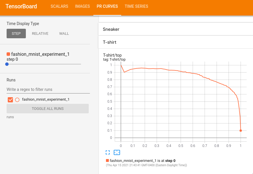
您现在可以看到 “PR Curves” 标签页，其中包含每个类别的精确率-召回率曲线。继续探索一下；您会看到对于某些类别，模型几乎达到100%的 “曲线下面积”（AUC），而对其他类别而言，这一面积较低：

这就是 TensorBoard 和其与 PyTorch集成的入门介绍。当然，您可以在 Jupyter Notebook 中完成所有 TensorBoard 提供的功能，但使用 TensorBoard，您可以获得默认即为交互式的可视化。